Functions
Euler’s method for an initial-value problem
1 2 3 4 5 6 7 8 9 10 11 12 13 14 15 16 17 18 19 20 21 22 23 24 25 26 27function [t,u] = eulersys(du_dt, tspan, u0, n) % EULERSYS Euler's method for a first-order IVP system. % Input: % du_dt defines f in u'(t) = f(t, u) % tspan endpoints of time interval (2-vector) % u0 initial value (m-vector) % n number of time steps (integer) % Output: % t selected nodes (vector, length n+1) % u solution values (array, n+1 by m) % Define the time discretization. a = tspan(1); b = tspan(2); h = (b - a) / n; t = a + (0:n)' * h; % Initialize solution array. u = zeros(length(u0), n+1); u(:, 1) = u0(:); % Time stepping. for i = 1:n u(:, i+1) = u(:, i) + h * du_dt(t(i), u(:, i)); end u = u.'; % conform to MATLAB output convention end
About the code
While the entries of u could be simplified to u(1), u(i), etc., we chose a column-access syntax like u(:, i) that will prove useful for what’s coming next in the chapter.
Improved Euler method for an IVP
1 2 3 4 5 6 7 8 9 10 11 12 13 14 15 16 17 18 19 20 21 22 23 24 25 26 27 28function [t, u] = ie2(du_dt, tspan, u0, n) % IE2 Improved Euler method for an IVP. % Input: % du_dt defines f in u'(t) = f(t, u) % tspan endpoints of time interval (2-vector) % u0 initial value (m-vector) % n number of time steps (integer) % Output: % t selected nodes (vector, length n+1) % u solution values (array, n+1 by m) % Define the time discretization. a = tspan(1); b = tspan(2); h = (b - a) / n; t = a + (0:n)' * h; % Initialize solution array. u = zeros(length(u0), n+1); u(:, 1) = u0(:); % Time stepping. for i = 1:n uhalf = u(:, i) + h/2 * du_dt(t(i), u(:, i)); u(:, i+1) = u(:, i) + h * du_dt(t(i) + h/2, uhalf); end u = u.'; % conform to MATLAB output convention end
Fourth-order Runge-Kutta for an IVP
1 2 3 4 5 6 7 8 9 10 11 12 13 14 15 16 17 18 19 20 21 22 23 24 25 26 27 28 29 30 31function [t, u] = rk4(du_dt, tspan, u0, n) % RK4 Fourth-order Runge-Kutta for an IVP. % Input: % du_dt defines f in u'(t) = f(t, u) % tspan endpoints of time interval (2-vector) % u0 initial value (m-vector) % n number of time steps (integer) % Output: % t selected nodes (vector, length n+1) % u solution values (array, n+1 by m) % Define the time discretization. a = tspan(1); b = tspan(2); h = (b - a) / n; t = a + (0:n)' * h; % Initialize solution array. u = zeros(length(u0), n+1); u(:, 1) = u0(:); % Time stepping. for i = 1:n k1 = h * du_dt( t(i), u(:, i) ); k2 = h * du_dt( t(i) + h/2, u(:, i) + k1/2); k3 = h * du_dt( t(i) + h/2, u(:, i) + k2/2); k4 = h * du_dt( t(i) + h, u(:, i) + k3 ); u(:, i+1) = u(:, i) + (k1 + 2*(k2 + k3) + k4) / 6; end u = u.'; % conform to MATLAB output convention end
Adaptive IVP solver based on embedded RK formulas
1 2 3 4 5 6 7 8 9 10 11 12 13 14 15 16 17 18 19 20 21 22 23 24 25 26 27 28 29 30 31 32 33 34 35 36 37 38 39 40 41 42 43 44 45 46 47 48 49 50 51function [t, u] = rk23(du_dt, tspan, u0, tol) % RK23 Adaptive IVP solver based on embedded RK formulas. % Input: % du_dt defines f in u'(t) = f(t, u) % tspan endpoints of time interval (2-vector) % u0 initial value (m-vector) % tol global error target (positive scalar) % Output: % t selected nodes (vector, length n+1) % u solution values (array, n+1 by m) % Initialize for the first time step. i = 1; t = tspan(1); u(:, 1) = u0(:); h = 0.5 * tol^(1/3); s1 = du_dt(t(1), u(:, 1)); % Time stepping. while t(i) < tspan(2) % Detect underflow of the step size. if t(i) + h == t(i) warning('Stepsize too small near t=%.6g.',t(i)) break % quit time stepping loop end % New RK stages. s2 = du_dt(t(i) + h/2, u(:, i) + (h/2) * s1); s3 = du_dt(t(i) + 3*h/4, u(:, i) + (3*h/4) * s2); unew2 = u(:, i) + h * (2*s1 + 3*s2 + 4*s3) / 9; % 2rd order solution s4 = du_dt(t(i) + h, unew2); err = h * (-5*s1/72 + s2/12 + s3/9 - s4/8); % 2nd/3rd order difference E = norm(err, Inf); % error estimate maxerr = tol * (1 + norm(u(:, i), Inf)); % relative/absolute blend % Accept the proposed step? if E < maxerr % yes t = [t; t(i) + h]; u(:, i+1) = unew2; i = i+1; s1 = s4; % use FSAL property end % Adjust step size. q = 0.8 * (maxerr / E) ^ (1/3); % optimal step factor q = min(q, 4); % limit stepsize growth h = min(q*h, tspan(2) - t(i)); % don't step past the end end u = u.'; % conform to MATLAB output convention end
About the code
The check t(i) + h == t(i)on line 24 is to detect when has become so small that it no longer changes the floating-point value of . This may be a sign that the underlying exact solution has a singularity near , but in any case, the solver must halt by using a break statement to exit the loop.
On line 36, we use a combination of absolute and relative tolerances to judge the acceptability of a solution value, as in (5.7.6). In lines 47--49 we underestimate the step factor a bit and prevent a huge increase in the step size, since a rejected step is expensive, and then we make sure that our final step doesn’t take us past the end of the domain.
Finally, line 43 exploits a subtle property of the BS23 formula called first same as last (FSAL).
While (6.5.5) calls for four stages to find the paired second- and third-order estimates, the final stage computed in stepping from to is identical to the first stage needed to step from to . By repurposing s4 as s1 for the next pass, one of the stage evaluations comes for free, and only three evaluations of are needed per successful step.
4th-order Adams–Bashforth formula for an IVP
1 2 3 4 5 6 7 8 9 10 11 12 13 14 15 16 17 18 19 20 21 22 23 24 25 26 27 28 29 30 31 32 33 34 35 36 37 38 39function [t, u] = ab4(du_dt, tspan, u0, n) %AB4 4th-order Adams-Bashforth formula for an IVP. % Input: % du_dt defines f in u'(t) = f(t, u) % tspan endpoints of time interval (2-vector) % u0 initial value (m-vector) % n number of time steps (integer) % Output: % t selected nodes (vector, length n+1) % u solution values (array, n+1 by m) % Define the time discretization. a = tspan(1); b = tspan(2); h = (b - a) / n; t = a + (0:n)' * h; % Constants in the AB4 method. k = 4; sigma = [55; -59; 37; -9] / 24; % Find starting values by RK4. u = zeros(length(u0), n+1); [~, us] = rk4(du_dt,[a, a + (k-1)*h], u0, k-1); u(:, 1:k) = us(1:k, :).'; % Compute history of u' values, from oldest to newest. f = zeros(length(u0), k); for i = 1:k-1 f(:, k-i) = du_dt(t(i), u(:, i)); end % Time stepping. for i = k:n f = [du_dt(t(i), u(:, i)), f(:, 1:k-1)]; % new value of du/dt u(:, i+1) = u(:, i) + h * (f * sigma); % advance one step end u = u.'; % conform to MATLAB output convention end
About the code
Line 21 sets sigma to be the coefficients of the generating polynomial of AB4. Lines 24--26 set up the IVP over the time interval , call rk4 to solve it using the step size , and use the result to fill the first four values of the solution. Then lines 29--32 compute the vector .
Line 36 computes , based on the most recent solution value and time. That goes into the first column of f, followed by the three values that were previously most recent. These are the four values that appear in (6.7.1). Each particular value starts at the front of f, moves through each position in the vector over three iterations, and then is forgotten.
2nd-order Adams–Moulton (trapezoid) formula for an IVP
1 2 3 4 5 6 7 8 9 10 11 12 13 14 15 16 17 18 19 20 21 22 23 24 25 26 27 28 29 30 31 32 33 34 35function [t, u] = am2(du_dt, tspan, u0, n) % AM2 2nd-order Adams-Moulton (trapezoid) formula for an IVP. % Input: % du_dt defines f in u'(t) = f(t, u) % tspan endpoints of time interval (2-vector) % u0 initial value (m-vector) % n number of time steps (integer) % Output: % t selected nodes (vector, length n+1) % u solution values (array, n+1 by m) % Define the time discretization. a = tspan(1); b = tspan(2); h = (b - a) / n; t = a + (0:n)' * h; u = zeros(length(u0), n+1); u(:, 1) = u0(:); % This function defines the rootfinding problem at each step. function F = trapzero(z) F = z - h/2 * du_dt(t(i+1), z) - known; end % Time stepping. for i = 1:n % Data that does not depend on the new value. known = u(:,i) + h/2 * du_dt(t(i), u(:, i)); % Find a root for the new value. unew = levenberg(@trapzero, known); u(:, i+1) = unew(:, end); end u = u.'; % conform to MATLAB output convention end % main function
About the code
Lines 32--34 define the function . This is sent to levenberg in line~27 to find the new solution value, using an Euler half-step as its starting value. A robust code would have to intercept the case where levenberg fails to converge, but we have ignored this issue for the sake of brevity.
Examples
6.1 Basics of IVPs
Example 6.1.2
Let’s use a built-in method to define and solve the initial-value problem
We must create a function that computes , an initial value for , and a vector describing the time domain.
f = @(t, u) sin((t + u)^2);
u0 = -1;
tspan = [0, 4];
These ingredients are supplied to a solver function. A standard first choice of solver is called ode45.
[t, u] = ode45(f, [0, 4], u0);
fprintf("length(t) = %d, length(u) = %d\n", length(t), length(u))
length(t) = 49, length(u) = 49
The solution is represented as a pair of vectors, t and u, where t contains the times at which the solution was computed and u contains the corresponding values of .
clf
plot(t, u, '-o')
xlabel("t")
ylabel("u(t)")
title(("Solution of an IVP"));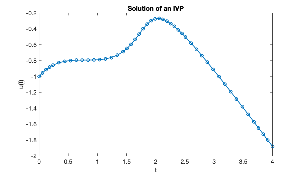
You might want to know the solution at particular times other than the ones selected by the solver. That requires an interpolation. To do this automatically requires calling the solver with just one output argument, which is then supplied to deval to evaluate the solution at any time.
sol = ode45(f, [0, 4], u0);
u = @(t) deval(sol, t)';    % return a column vector
u(0:0.5:2)Example 6.1.3
The equation gives us some trouble.
f = @(t, u) (t + u)^2;
u0 = 1;
tspan = [0, 1];
[t, u] = ode45(f, tspan, u0);
Warning: Failure at t=7.853789e-01. Unable to meet integration tolerances without reducing the step size below the smallest value allowed (1.776357e-15) at time t.The warning message we received can mean that there is a bug in the formulation of the problem. But if everything has been done correctly, it suggests that the solution simply may not exist past the indicated time. This is a possibility in nonlinear ODEs.
clf
semilogy(t, u)
xlabel("t")
ylabel("u(t)")
title(("Finite-time blowup"));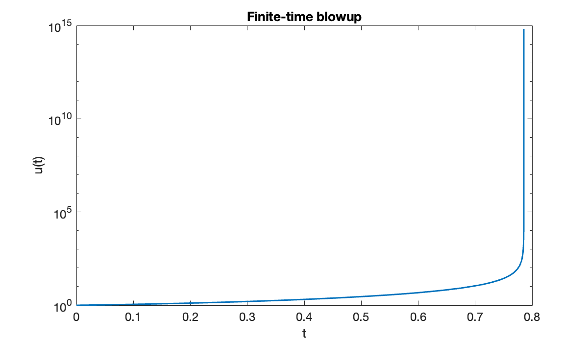
Example 6.1.5
Consider the ODEs and . In each case we compute , so the condition number bound from Theorem 6.1.2 is in both problems. However, they behave quite differently. In the case of exponential growth, , the bound is the actual condition number.
Source
clf
for u0 = [0.7, 1, 1.3]    % initial values
    fplot(@(t) exp(t) * u0, [0, 3]), hold on
end
xlabel('t')
ylabel('u(t)')
title(('Exponential divergence of solutions'));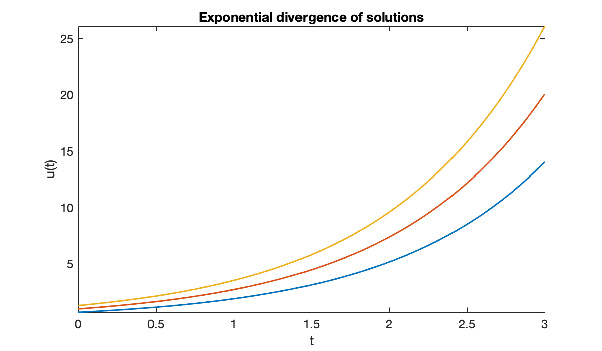
But with , solutions actually get closer together with time.
Source
clf
for u0 = [0.7, 1, 1.3]    % initial values
    fplot(@(t) exp(-t) * u0, [0, 3]), hold on
end
xlabel('t')
ylabel('u(t)')
title(('Exponential convergence of solutions'));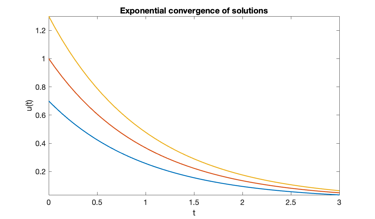
In this case the actual condition number is one, because the initial difference between solutions is the largest over all time. Hence the exponentially growing bound is a gross overestimate.
6.2 Euler’s method
Example 6.2.1
We consider the IVP
As usual, we need to define the function for the right-hand side of the ODE, the interval for the independent variable, and the initial value.
f = @(t, u) sin((t + u)^2);
u0 = -1;
tspan = [0, 4];
Here is the call to Function 6.2.1.
[t, u] = eulersys(f, tspan, u0, 20);
clf, plot(t, u, '.-', displayname='20 steps')
xlabel('t')
ylabel('u(t)')
title(('Solution by Euler''s method'));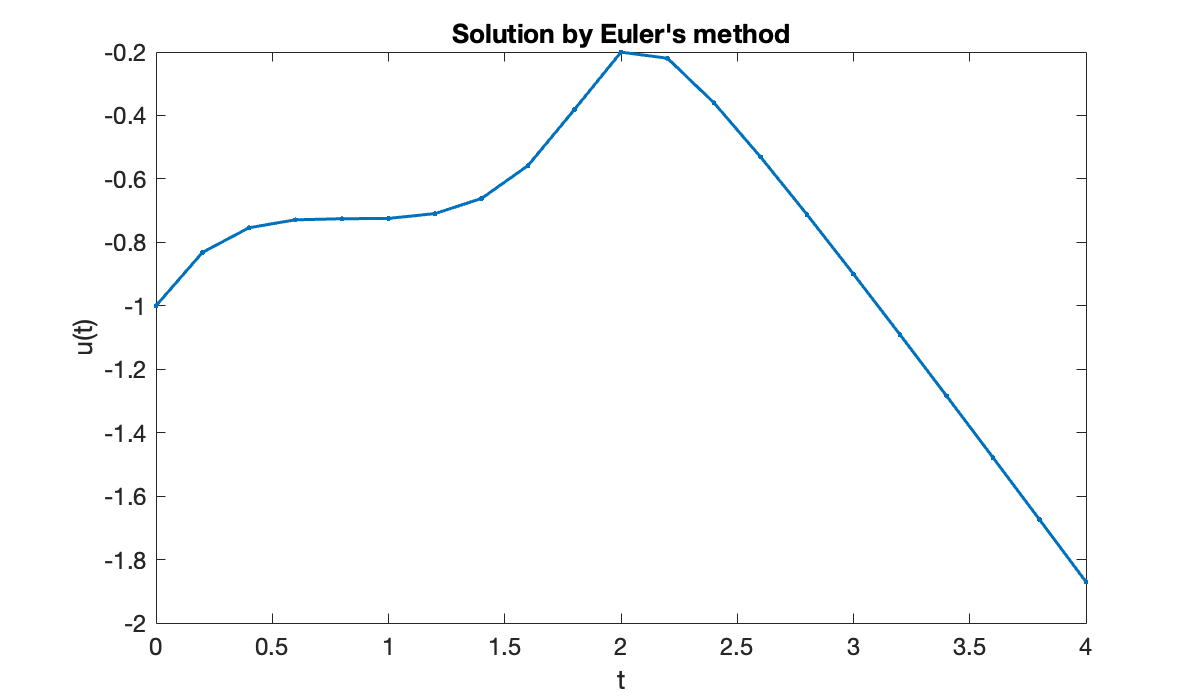
We could define a different interpolant to get a smoother picture above, but the derivation of Euler’s method assumed a piecewise linear interpolant, and that sets the limit of its accuracy. We can instead request more steps to make the interpolant look smoother.
[t, u] = eulersys(f, tspan, u0, 50);
hold on, plot(t, u, '.-',  displayname='50 steps')
legend();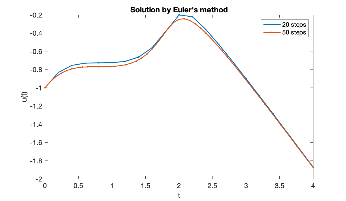
Increasing changed the solution noticeably. Since we know that interpolants and finite differences become more accurate as , we should anticipate the same behavior from Euler’s method. We don’t have an exact solution to compare to, so we will use a built-in solver to construct an accurate reference solution.
opt = odeset('RelTol', 1e-13, 'AbsTol', 1e-13);
sol = ode45(f, tspan, u0, opt);
u_ref = @(t) deval(sol, t)';
Now we can perform a convergence study.
n = round(5 * 10.^(0:0.5:3));
err = [];
for k = 1:length(n)
    [t, u] = eulersys(f, tspan, u0, n(k));
    err(k) = norm(u_ref(t) - u, Inf);
end
table(n', err', VariableNames=["n", "inf-norm error"])The error is approximately cut by a factor of 10 for each increase in by the same factor. A log-log plot also confirms first-order convergence. Keep in mind that since , it follows that .
clf
loglog(n, err, 'o-')
hold on, loglog(n, 0.5 * err(end) * (n / n(end)).^(-1), '--')
xlabel('n')
ylabel('inf-norm error')
title('Convergence of Euler''s method')
legend('error', 'O(n^{-1})', 'location', 'southwest');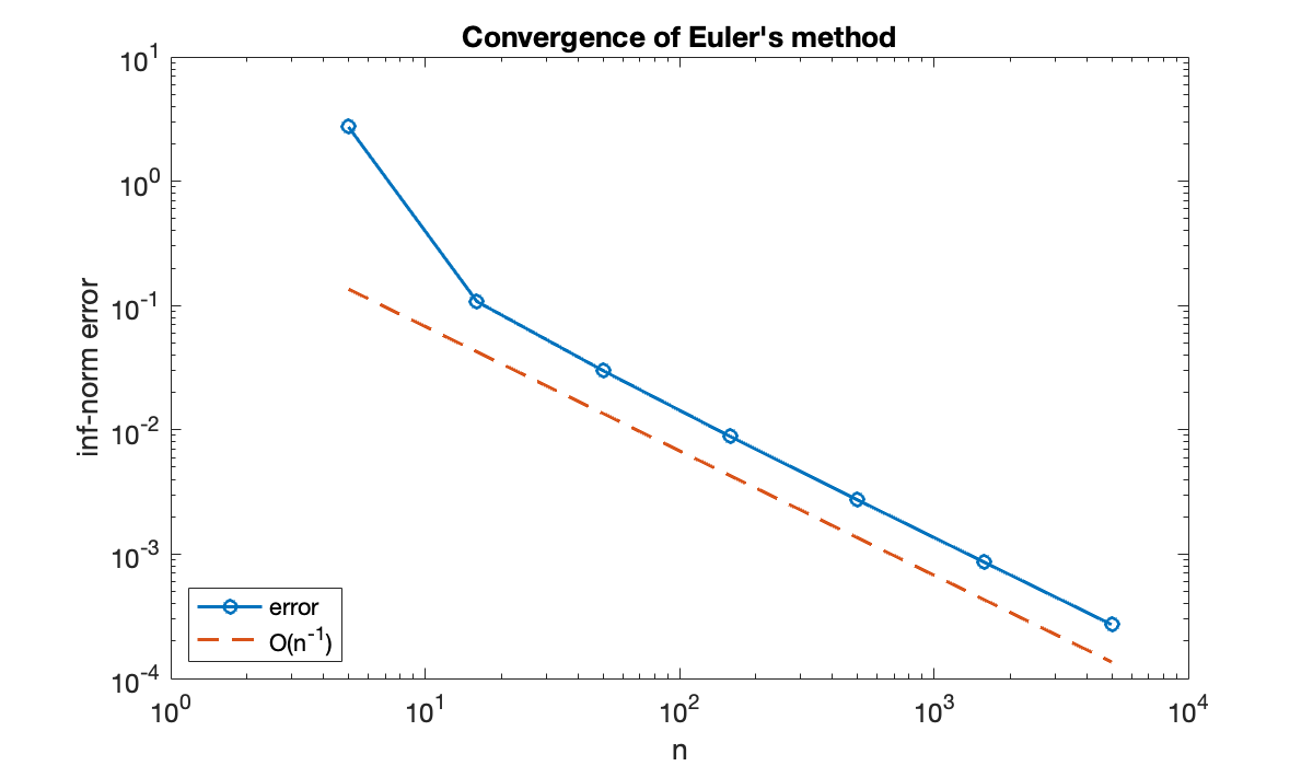
6.3 IVP systems
Example 6.3.2
We encode the predator–prey equations via a function, defined here externally.
function du_dt = predprey(t, u, p)
    alpha = p(1);  beta = p(2);
    y = u(1);      z = u(2);
    s = (y * z) / (1 + beta * y);  % appears in both equations
    du_dt = [ y * (1 - alpha * y) - s;  -z + s ];
end
The values of alpha and beta are parameters that influence the solution of the IVP, so the function signature above includes a third argument for them. But the solvers we use expect to receive a function of and only. To deal with this, we create a function handle f that captures the parameter values in its definition.
params = [0.1, 0.25];
f = @(t, u) f63_predprey(t, u, params);
Tip
The technique above is called currying or partial application. If we later want to change the values of the parameters, we have to redefine f with the new values.
We use a new syntax here for calling ode45. By giving it a vector as the tspan argument, we are asking it to return the solution at the times in that vector.
u0 = [1; 0.01];    % column vector
a = 0; b = 60;     % time interval

[t, u] = ode45(f, linspace(a, b, 1001), u0);
size(u)Each row of u from the output is the solution vector at a particular time; each column is a component of over all time.
clf
plot(t, u)
xlabel("t")
ylabel("u(t)")
title('Predator-prey solution')
legend('prey', 'predator');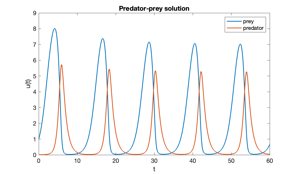
We can also use Function 6.2.1 to find the solution (although it does not allow us to choose different time nodes for the output).
[t_e, u_e] = eulersys(f, [a, b], u0, 1200);hold on
plot(t_e, u_e, '.', displayname='Euler')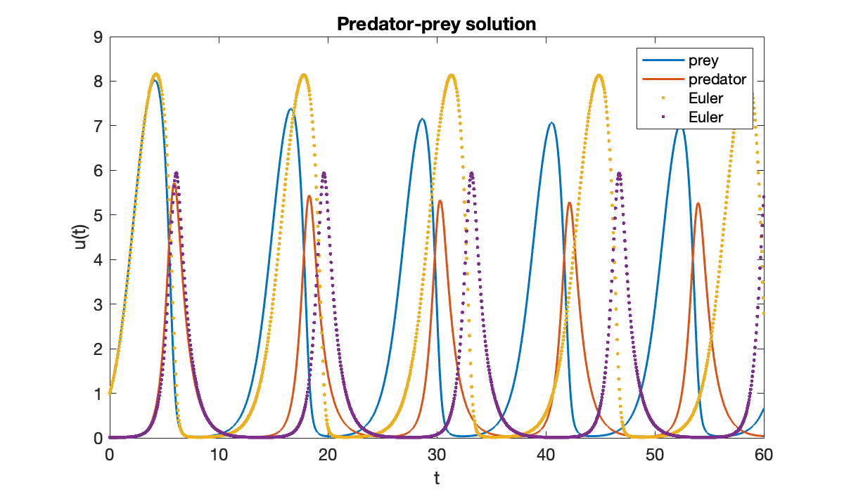
Notice above that the accuracy of the Euler solution deteriorates rapidly.
When there are just two components, it’s common to plot the solution in the phase plane, i.e., with and along the axes and time as a parameterization of the curve.
clf
plot(u(:, 1), u(:, 2))
title("Predator-prey solution in the phase plane")
xlabel("prey, y(t)")
ylabel("predator, z(t)");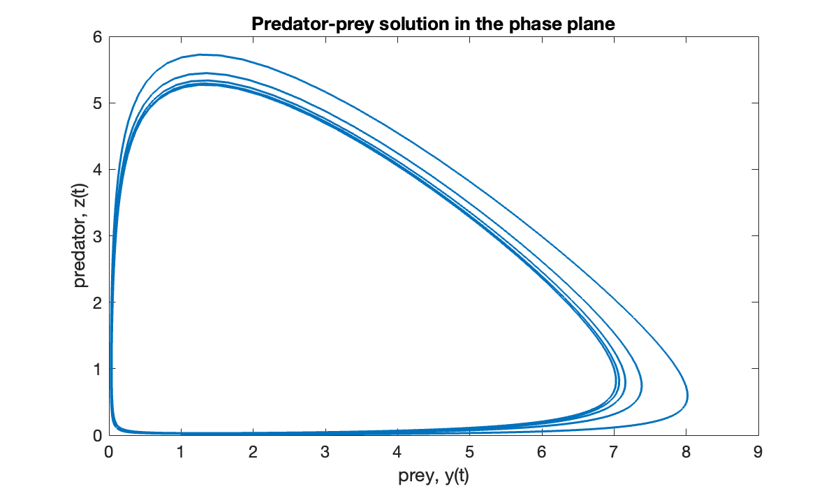
As time progresses, the point in the phase plane spirals inward toward a limiting closed loop called a limit cycle representing a periodic solution:
Source
axis(axis)
cla,  hold on
grid on
curve_ = plot(u(1, 1), u(1, 2))
head_ = plot(u(1, 1), u(1, 2), 'o', 'markersize', 10, 'markerfacecolor', 'r');
title('Predator–prey solution in the phase plane')
xlabel("prey, y(t)")
ylabel("predator, z(t)");
vid = VideoWriter("figures/predator-prey.mp4","MPEG-4");
vid.Quality = 85;
open(vid)
for frame = 1:2:length(t)
    curve_.XData = u(1:frame, 1);
    curve_.YData = u(1:frame, 2);
    head_.XData = u(frame, 1);
    head_.YData = u(frame, 2);
    writeVideo(vid, frame2im(getframe(gcf)));
end
close(vid)Example 6.3.5
Let’s implement the coupled pendulums from Example 6.3.4. The pendulums will be pulled in opposite directions and then released together from rest.
function udot = pendulums(t, u, p)
    gamma = p(1);  L = p(2);  k = p(3);
    g = 9.8;
    udot = zeros(4, 1);
    udot(1:2) = u(3:4);
    udot(3) = -gamma * u(3) - (g / L) * sin(u(1)) + k * (u(2) - u(1));
    udot(4) = -gamma * u(4) - (g / L) * sin(u(2)) + k * (u(1) - u(2));
end
u0 = [1.25; -0.3; 0; 0];
tspan = [0, 50];
First we check the behavior of the system when the pendulums are uncoupled, i.e., when .
Tip
A third argument to deval is used below to restrict output to just and .
params =[0.01, 0.5, 0];    % gamma, L, k
f = @(t, u) f63_pendulums(t, u, params);
sol = ode45(f, tspan, u0);
theta = @(t) deval(sol, t, 1:2)';
t = linspace(tspan(1), tspan(2), 901);
clf, plot(t, theta(t))
xlabel("t");  ylabel("angle")
title("Uncoupled pendulums")
legend("\theta_1", "\theta_2");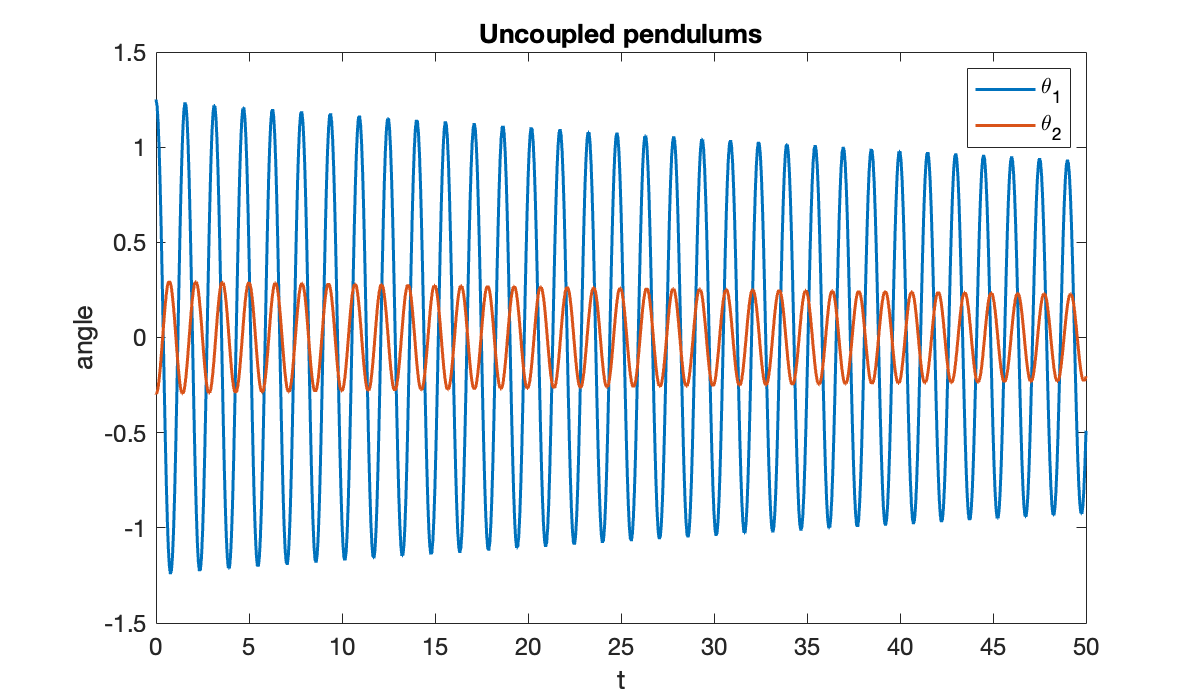
You can see that the pendulums swing independently:
Source
clf
rod_ = [];  bob_ = [];
for k = 1:2
    subplot(1, 2, k)
    axis equal, axis([-1.1, 1.1, -1.1, 1.1])
    hold on, axis off
    rod_ = [rod_; plot(0, 0, 'linewidth', 3)];
    bob_= [bob_; plot(0, 0, 'ko', 'markersize', 20, 'markerfacecolor', 'k')];
end
text_ = text(-0.9, 0.85, "t = 0", 'fontsize', 20);
vid = VideoWriter("figures/pendulums-weak.mp4","MPEG-4");
vid.FrameRate = 24;
open(vid)
for frame = 1:401
    q = theta(t(frame));
    for k = 1:2
        rod_(k).XData = [0, sin(q(k))];
        rod_(k).YData = [0, -cos(q(k))];
        bob_(k).XData = sin(q(k));
        bob_(k).YData = -cos(q(k));
    end
    text_.String = sprintf("t = %.2f", t(frame));
    writeVideo(vid, frame2im(getframe(gcf)));
end
close(vid)
Because the model is nonlinear and the initial angles are not small, they have slightly different periods of oscillation, and they go in and out of phase.
With coupling activated, a different behavior is seen.
params(3) = 1;
f = @(t, u) f63_pendulums(t, u, params);
sol = ode45(f, tspan, u0);
theta = @(t) deval(sol, t, 1:2)';
clf, plot(t, theta(t))
xlabel("t");  ylabel("angle")
title("Coupled pendulums")
legend("\theta_1", "\theta_2");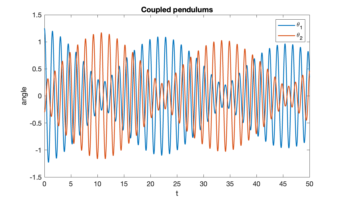
The coupling makes the pendulums swap energy back and forth:
Source
clf
rod_ = [];  bob_ = [];
for k = 1:2
    subplot(1, 2, k)
    axis equal, axis([-1.1, 1.1, -1.1, 1.1])
    hold on, axis off
    rod_ = [rod_; plot(0, 0, 'linewidth', 3)];
    bob_= [bob_; plot(0, 0, 'ko', 'markersize', 20, 'markerfacecolor', 'k')];
end
text_ = text(-0.9, 0.85, "t = 0", 'fontsize', 20);
vid = VideoWriter("figures/pendulums-strong.mp4","MPEG-4");
vid.FrameRate = 24;
open(vid)
for frame = 1:length(t)
    q = theta(t(frame));
    for k = 1:2
        rod_(k).XData = [0, sin(q(k))];
        rod_(k).YData = [0, -cos(q(k))];
        bob_(k).XData = sin(q(k));
        bob_(k).YData = -cos(q(k));
    end
    text_.String = sprintf("t = %.2f", t(frame));
    writeVideo(vid, frame2im(getframe(gcf)));
end
close(vid)
6.4 Runge–Kutta methods
Example 6.4.1
We solve the IVP
f = @(t, u) sin((t + u)^2);
u0 = -1;
a = 0;  b = 4;
We use a built-in solver to construct an accurate approximation to the exact solution.
opt = odeset('RelTol', 1e-13, 'AbsTol', 1e-13);
sol_ref = ode45(f, [a, b], u0, opt);
u_ref = @(t) deval(sol_ref, t)';
Now we perform a convergence study of our two Runge–Kutta implementations.
n = round(2 * 10.^(0:0.5:3)');
err = zeros(length(n), 2);
for i = 1:length(n)
    [t, u] = ie2(f, [a, b], u0, n(i));
    err(i, 1) = norm(u_ref(t) - u, Inf);
    [t, u] = rk4(f, [a, b], u0, n(i));
    err(i, 2) = norm(u_ref(t) - u, Inf);
end

table(n, err(:, 1), err(:, 2), variableNames=["n", "IE2 error", "RK4 error"])The amount of computational work at each time step is assumed to be proportional to the number of stages. Let’s compare on an apples-to-apples basis by using the number of -evaluations on the horizontal axis.
clf, loglog([2*n 4*n], err, '-o')
hold on
loglog(2*n, 1e-5 * (n / n(end)) .^ (-2), '--')
loglog(4*n, 1e-10 * (n / n(end)) .^ (-4), '--')
xlabel("f-evaluations");  ylabel("inf-norm error")
title("Convergence of RK methods")
legend("IE2", "RK4", "O(n^{-2})", "O(n^{-4})", "location", "southwest");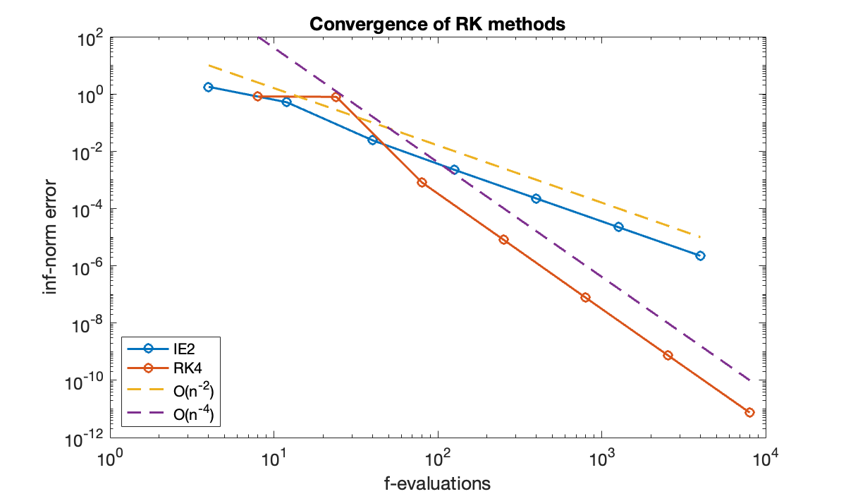
The fourth-order variant is more efficient in this problem over a wide range of accuracy.
6.5 Adaptive Runge–Kutta
Example 6.5.1
Let’s run adaptive RK on .
f = @(t, u) exp(t - u * sin(u));
u0 = 0;
a = 0;  b = 5;

[t, u] = rk23(f, [a, b], u0, 1e-5);
clf, plot(t, u)
xlabel("t");  ylabel("u(t)")
title(("Adaptive IVP solution"));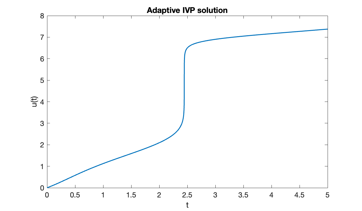
The solution makes a very abrupt change near . The resulting time steps vary over three orders of magnitude.
Delta_t = diff(t);
semilogy(t(1:end-1), Delta_t)
xlabel("t");  ylabel("step size")
title(("Adaptive step sizes"));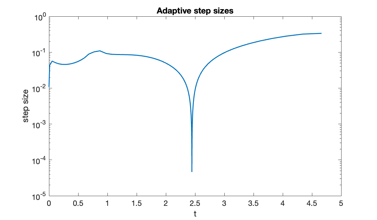
If we had to run with a uniform step size to get this accuracy, it would be
fprintf("minimum step size = %.2e", min(Delta_t))minimum step size = 4.61e-05On the other hand, the average step size that was actually taken was
fprintf("average step size = %.2e", mean(Delta_t))average step size = 3.21e-02We took fewer steps by a factor of almost 1000! Even accounting for the extra stage per step and the occasional rejected step, the savings are clear.
Example 6.5.2
In Example 6.1.3 we saw an IVP that appears to blow up in a finite amount of time. Because the solution increases so rapidly as it approaches the blowup, adaptive stepping is required even to get close.
f = @(t, u) (t + u)^2;
u0 = 1;
[t, u] = rk23(f, [0, 1], u0, 1e-5);
Warning: Stepsize too small near t=0.785409.In fact, the failure of the adaptivity gives a decent idea of when the singularity occurs.
clf, semilogy(t, u)
xlabel("t");  ylabel("u(t)")
title("Adaptive solution near a singularity")

tf = t(end);
xline(tf, "linestyle", "--")
text(tf, 1e5, sprintf(" t = %.6f ", tf))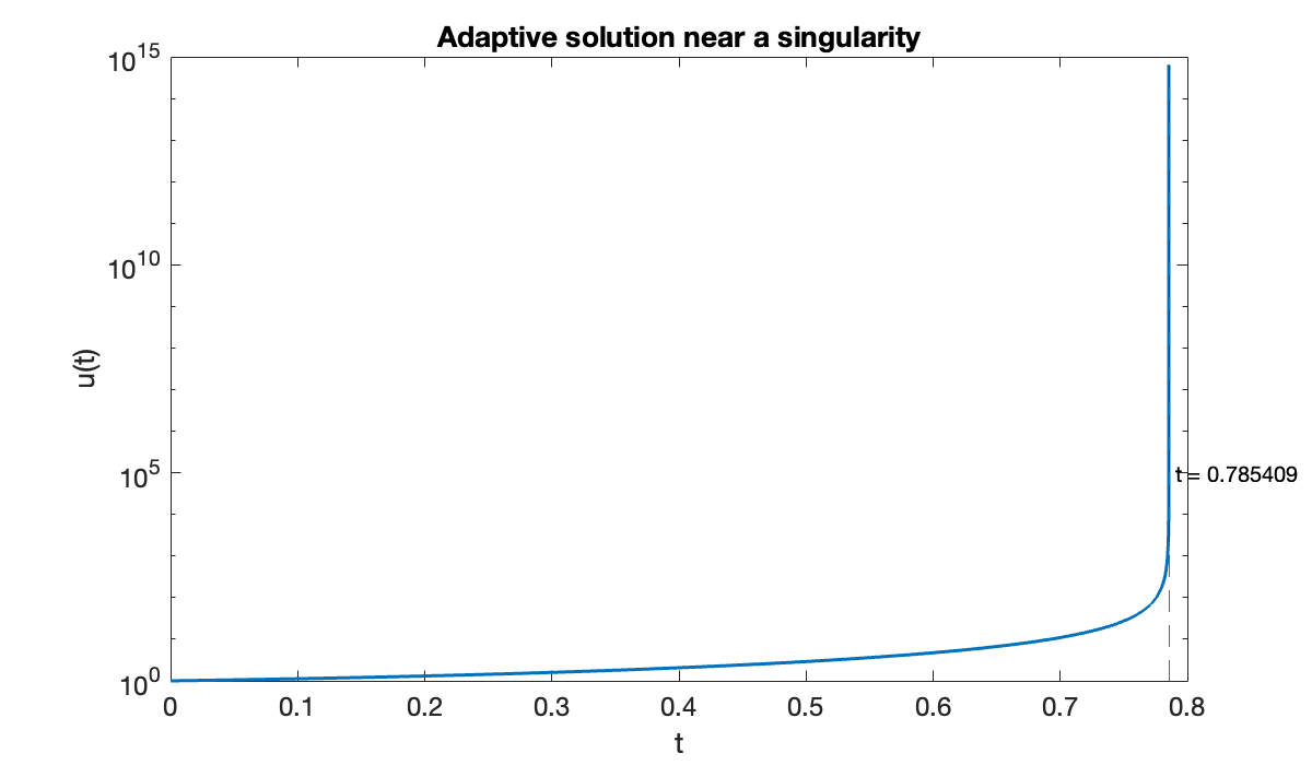
6.7 Multistep methods
Example 6.7.1
We study the convergence of AB4 using the IVP over , with . As usual, a built-in solver is called to give an accurate reference solution.
f = @(t, u) sin((t + u)^2);
u0 = -1;
a = 0;  b = 4;
opt = odeset('RelTol', 1e-13, 'AbsTol', 1e-13);
sol_ref = ode45(f, [a, b], u0, opt);
u_ref = @(t) deval(sol_ref, t)';
Now we perform a convergence study of the AB4 code.
n = round(4 * 10.^(0:0.5:3)');
err = zeros(size(n));
for i = 1:length(n)
    [t, u] = ab4(f, [a, b], u0, n(i));
    err(i) = norm(u_ref(t) - u, Inf);
end
table(n, err, variableNames=["n", "inf-norm error"])The method should converge as , so a log-log scale is appropriate for the errors.
clf, loglog(n, err, '-o')
hold on
loglog(n, 0.5 * err(end) * (n / n(end)) .^ (-4), '--')
xlabel("n");  ylabel("inf-norm error")
title("Convergence of AB4")
legend("AB4", "O(n^{-4})", location="southwest");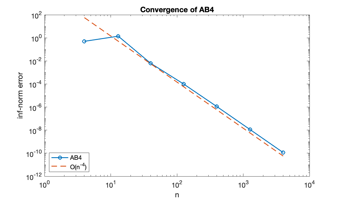
Example 6.7.2
The following simple ODE uncovers a surprise.
f = @(t, u) u^2 - u^3;
u0 = 0.005;
We will solve the problem first with the implicit AM2 method using steps.
[tI, uI] = am2(f, [0, 400], u0, 200);
clf
plot(tI, uI)
xlabel("t");  ylabel(("u(t)"));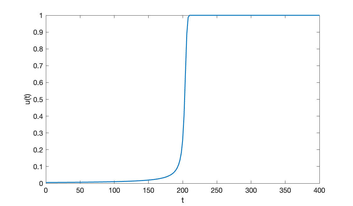
Now we repeat the process using the explicit AB4 method.
[tE, uE] = ab4(f, [0, 400], u0, 200);
hold on
plot(tE, uE, '.', 'markersize', 8)
ylim([-5, 3])
legend("AM2", "AB4");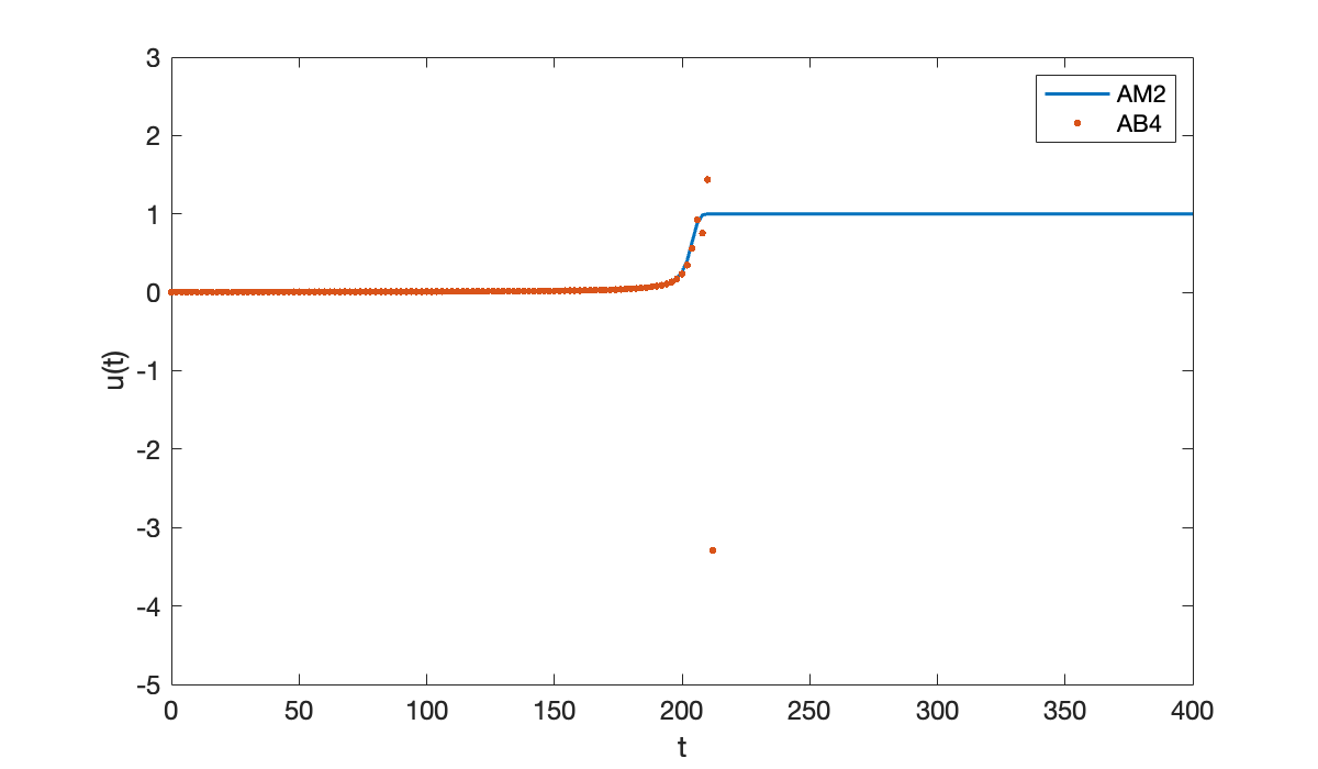
Once the solution starts to take off, the AB4 result goes catastrophically wrong.
format short e
uE(105:111)We hope that AB4 will converge in the limit , so let’s try using more steps.
clf,  plot(tI, uI, '.', 'markersize', 10)
hold on
[tE, uE] = ab4(f, [0, 400], u0, 1000);
plot(tE, uE)
[tE, uE] = ab4(f, [0, 400], u0, 1600);
plot(tE, uE)
legend("AM2, n=200", "AB4, n=1000", "AB4, n=1600", location="northwest");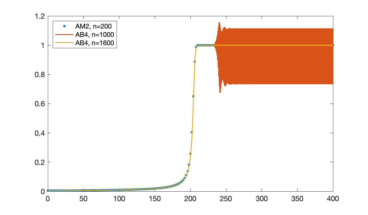
So AB4, which is supposed to be more accurate than AM2, actually needs something like 8 times as many steps to get a reasonable-looking answer!
6.8 Implementation of multistep methods
Example 6.8.1
We’ll measure the error at the time .
du_dt = @(t, u) u;
u_exact = @exp;
a = 0;  b = 1;
n = [5, 10, 20, 40, 60]';
err = zeros(size(n));
for j = 1:length(n)
    h = (b - a) / n(j);
    t = a + h *(0:n(j));
    u = [1, u_exact(h), zeros(1, n(j) - 1)];
    f = [du_dt(t(1), u(1)), zeros(1, n(j) - 2)];
    for i = 2:n(j)
        f(i) = du_dt(t(i), u(i));
        u(i+1) = -4*u(i) + 5*u(i-1) + h * (4*f(i) + 2*f(i-1));
    end
    err(j) = abs(u_exact(b) - u(end));
end

h = (b-a) ./ n;
table(n, h, err)The error starts out promisingly, but things explode from there. A graph of the last numerical attempt yields a clue.
clf
semilogy(t, abs(u))
xlabel("t");  ylabel("|u(t)|")
title(("LIAF solution"));
It’s clear that the solution is growing exponentially in time.