Chapter 13 - Fundamentals of Numerical Computation

Functions¶

Create a tensor-product grid

tensorgrid.m

1
2
3
4
5
6
7
8
9
10
11
12
13
14
15
16
17
18
19
20
21
22
23
24
25
26
27
function [mtx, X, Y, vec, unvec, is_boundary] = tensorgrid(x, y)
% TENSORGRID Tensor-product grid.
% Input:
%   x, y           1d projections of the grid nodes (lengths m and n)
% Output:
%   mtx            evaluate a function on the grid (function)
%   X, Y           mtx applied to the coordinate functions (m×n)
%   vec            convert grid shape to vector shape (function)
%   unvec          convert vector shape to grid shape (function)
%   is_boundary    indicator of boundary nodes (logical m×n)
    m = length(x) - 1;
    n = length(y) - 1;
    vec = @(U) U(:);
    unvec = @(u) reshape(u, m+1, n+1);
    [X, Y] = ndgrid(x, y);
    function F = grideval(f)
        F = zeros(size(X));
        for k = 1:numel(X)
            F(k) = f(X(k), Y(k));
        end
    end
    mtx = @grideval;
    
    % Identify boundary points.
    is_boundary = true(m+1, n+1);
    is_boundary(2:m, 2:n) = false;
end

Solution of Poisson’s equation by finite differences

poissonfd.m

1
2
3
4
5
6
7
8
9
10
11
12
13
14
15
16
17
18
19
20
21
22
23
24
25
26
27
28
29
30
31
32
33
34
35
function [X, Y, U] = poissonfd(f, g, m, xspan, n, yspan)
%POISSONFD   Solve Poisson's equation by finite differences.
% Input:
%   f            forcing function (function of x, y)
%   g            boundary condition (function of x, y)
%   m            number of grid points in x (integer)
%   xspan        endpoints of the domain of x (2-vector)
%   n            number of grid points in y (integer)
%   yspan        endpoints of the domain of y (2-vector)
%
% Output:
%   U            solution (m+1 by n+1)
%   X,Y          grid matrices (m+1 by n+1)

    % Discretize the domain.
    [x, Dx, Dxx] = diffmat2(m, xspan);
    [y, Dy, Dyy] = diffmat2(n, yspan);
    [mtx, X, Y, vec, unvec, is_boundary] = tensorgrid(x, y);

    % Form the collocated PDE as a linear system. 
    Ix = speye(m+1);  Iy = speye(n+1);
    A = kron(Iy, sparse(Dxx)) + kron(sparse(Dyy), Ix);  % Laplacian matrix
    b = vec(mtx(f));

    % Replace collocation equations on the boundary.
    scale = max(abs(A(n + 2, :)));
    I = speye(size(A));
    idx = vec(is_boundary);
    A(idx, :) = scale * I(idx, :);           % Dirichet assignment
    b(idx) = scale * g( X(idx), Y(idx) );     % assigned values

    % Solve the linear sytem and reshape the output.
    u = A \ b;
U = unvec(u);
end

Solution of elliptic PDE by Chebyshev collocation

elliptic.m

1
2
3
4
5
6
7
8
9
10
11
12
13
14
15
16
17
18
19
20
21
22
23
24
25
26
27
28
29
30
31
32
33
34
35
36
37
38
39
40
41
42
43
44
45
46
47
48
49
50
51
52
53
54
55
function u = elliptic(phi, g, m, xspan, n, yspan)
%ELLIPTIC   Solve an elliptic PDE in 2d.
% Input:
%   phi          defines phi(x, y, u, u_x, u_xx, u_y, u_yy) = 0 (function)
%   g            boundary condition (function)
%   m, xspan     size and interval of x discretization (integer, 2-vector)
%   n, yspan     size and interval of y discretization (integer, 2-vector)
% Output:
%   U            solution (n+1 by n+1)
%   X,Y          coordinate matrices (n+1 by n+1)

    % Discretize the domain.
    [x, Dx, Dxx] = diffcheb(m, xspan);
    [y, Dy, Dyy] = diffcheb(n, yspan);
    [mtx, X, Y, vec, unvec, is_boundary] = tensorgrid(x, y);

    % Identify boundary locations and evaluate the boundary condition.
    idx = vec(is_boundary);
    gb = g(X(idx), Y(idx));

    % Evaluate the PDE+BC residual.
    function r = residual(u)
        U = unvec(u);
        R = phi(X, Y, U, Dx * U, Dxx * U, U * Dy', U * Dyy');  % PDE
        R(idx) = u(idx) - gb;                                  % boundary
        r = vec(R);
    end

    % Solve the equation.
    u = levenberg(@residual, vec(zeros(size(X))));
    U = unvec(u(:, end));

    function u = evaluate(xi, eta)
        v = zeros(1, n+1);
        for j = 1:n+1
            v(j) = chebinterp(x, U(:, j), xi);
        end
        u = chebinterp(y, v, eta);
    end

    u = @evaluate;
end

function f = chebinterp(x, v, xi)
    n = length(x) - 1;
    w = (-1.0) .^ (0:n)';
    w([1, n+1]) = w([1, n+1]) / 2;

    terms = w ./ (xi - x(:));
    if any(isinf(terms))     % exactly at a node
        f = v(xi == x);
    else
        f = sum(v(:) .* terms) / sum(terms);
    end
end

Examples¶

13.1 Tensor-product discretizations¶

Example 13.1.2

Here is the grid from Example 13.1.1.

m = 4;   
x = linspace(0, 2, m+1);
n = 2;   
y = linspace(1, 3, n+1);

For a given $f(x,y)$ we can find $\operatorname{mtx}(f)$ by using a comprehension syntax.

[mtx, X, Y] = tensorgrid(x, y);
f = @(x, y) cos(pi * x .* y - y);
F = mtx(f)

We can make a nice plot of the function by first choosing a much finer grid. However, the contour and surface plotting functions expect the transpose of mtx( $f$ ).

m = 80;  x = linspace(0, 2, m+1);
n = 60;  y = linspace(1, 3, n+1);
[mtx, X, Y] = tensorgrid(x, y);
F = mtx(f);

pcolor(X', Y', F')
shading interp
colormap(redsblues),  colorbar
axis equal
xlabel("x"),  ylabel("y")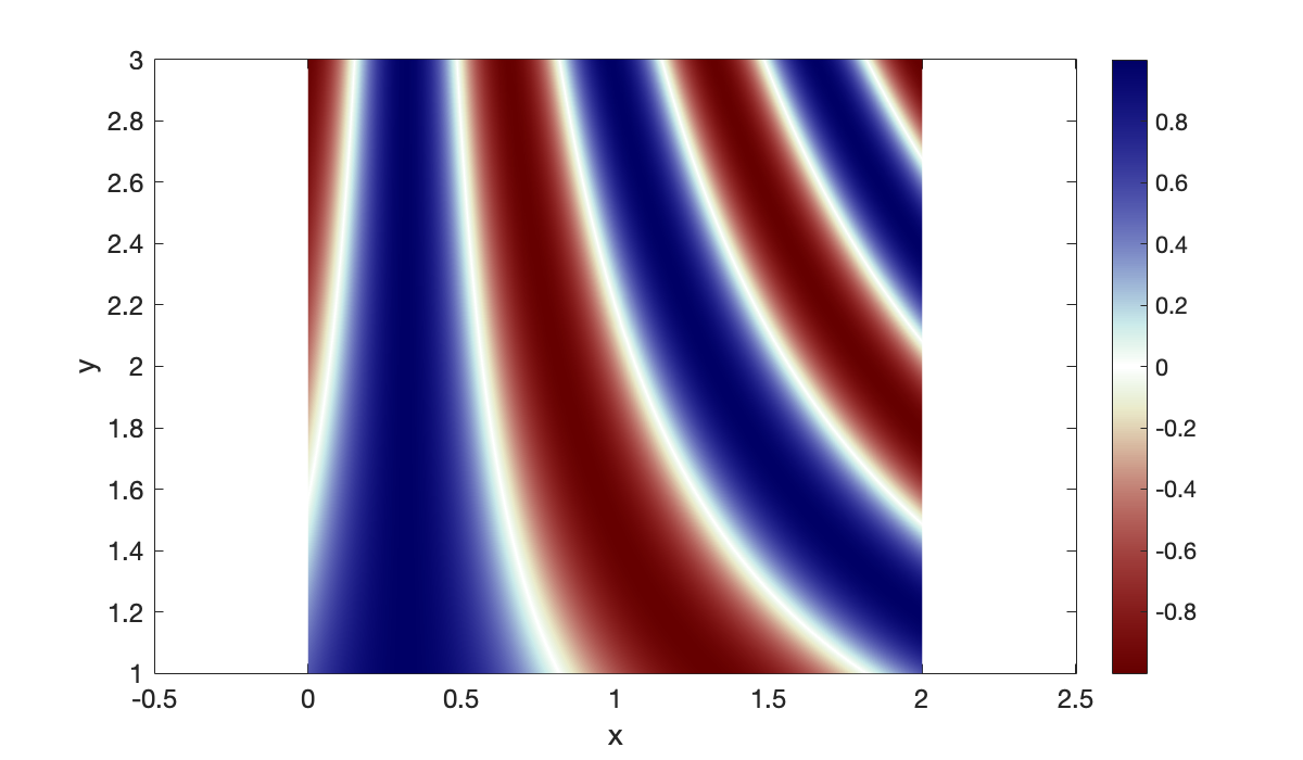

Example 13.1.3

For a function given in polar form, such as $f(r,\theta)=1-r^4$ , construction of a function over the unit disk is straightforward using a grid in $(r,\theta)$ space.

r = linspace(0, 1, 41);
theta = linspace(0, 2*pi, 121);
[mtx, R, Theta] = tensorgrid(r, theta);
F = mtx(@(r, theta) 1 - r.^4);
clf,  colormap(parula)
contourf(R', Theta', F', 20)
shading flat
xlabel("r"),  ylabel("\theta"), 
title("A polar function")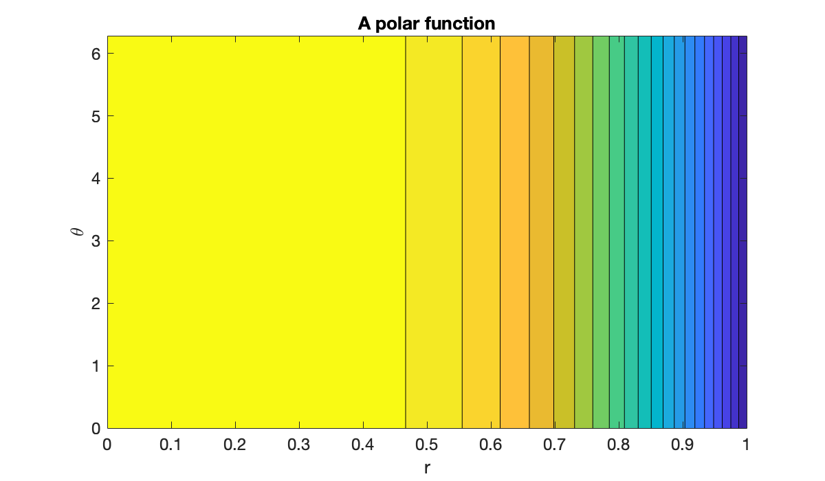

Of course, we are used to seeing such plots over the $(x,y)$ plane, not the $(r,\theta)$ plane. For this we create matrices for the coordinate functions $x$ and $y$ .

X = R .* cos(Theta);  Y = R .* sin(Theta);
contourf(X', Y', F', 20)
axis equal,  shading interp  
xlabel('x'),  ylabel('y')
title('Function over the unit disk')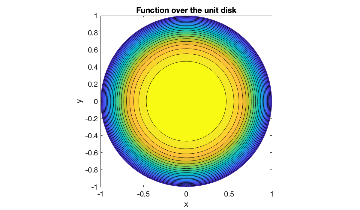

In such functions the values along the line $r=0$ must be identical, and the values on the line $\theta=0$ should be identical to those on $\theta=2\pi$ . Otherwise the interpretation of the domain as the unit disk is nonsensical. If the function is defined in terms of $x$ and $y$ , then those can be defined in terms of $r$ and θ using (13.1.5).

Example 13.1.4

We define a function and, for reference, its two exact partial derivatives.

u = @(x, y) sin(pi * x .* y - y);
du_dx = @(x, y) pi * y .* cos(pi * x .* y - y);
du_dy = @(x, y) (pi * x - 1) .* cos(pi * x .* y - y);

We will use an equispaced grid and second-order finite differences as implemented by diffmat2.

m = 80;  [x, Dx] = diffmat2(m, [0, 2]);
n = 70;  [y, Dy] = diffmat2(n, [1, 3]);
[mtx, X, Y] = tensorgrid(x, y);
U = mtx(u);
dU_dX = mtx(du_dx);
dU_dY = mtx(du_dy);

First, we have a look at a plots of the exact partial derivatives.

clf,  subplot(1, 2, 1)
pcolor(X', Y', dU_dX')
axis equal,  shading interp
title('∂u/∂x')
subplot(1, 2, 2)
pcolor(X', Y', dU_dY')
axis equal,  shading interp
title('∂u/∂y')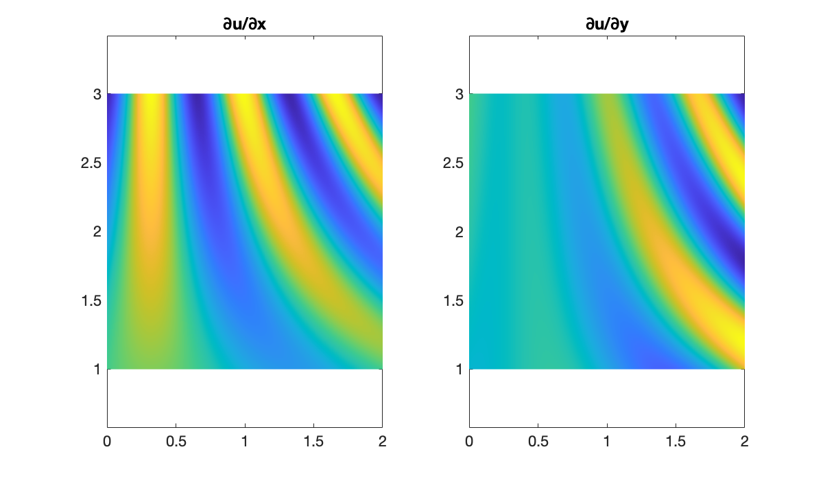

Now we compare the exact partial derivatives with their finite-difference approximations. Since these are signed errors, we use a colormap that is symmetric around zero.

err = dU_dX - Dx * U;
subplot(1, 2, 1)
M = max(abs(err(:)));
pcolor(X', Y', err')
colorbar,  clim([-M, M])
axis equal,  shading interp
title('error in ∂u/∂x')

err = dU_dY - U * Dy';
subplot(1,2,2)
M = max(abs(err(:)));
pcolor(X', Y', err')
colorbar,  clim([-M, M])
axis equal,  shading interp
colormap(redsblues)
title('error in ∂u/∂y')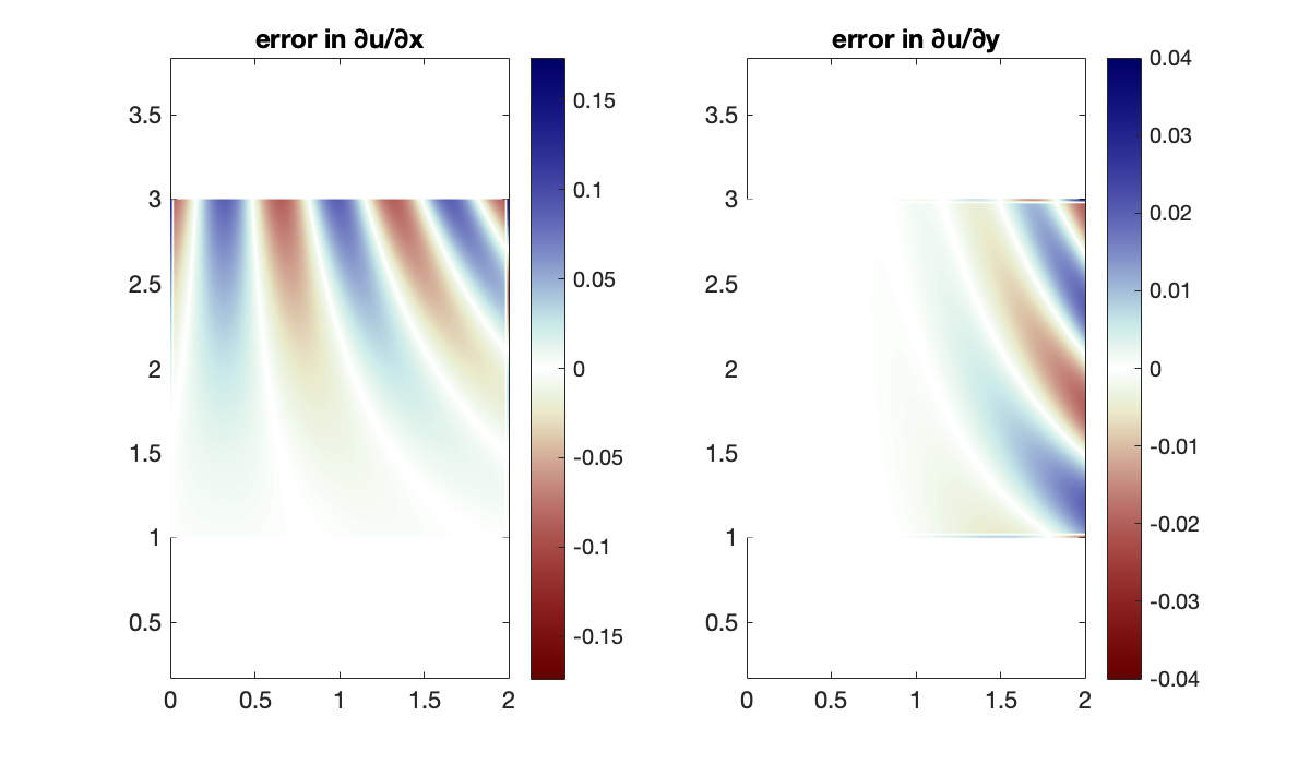

Not surprisingly, the errors are largest where the derivatives themselves are largest.

13.2 Two-dimensional diffusion and advection¶

Example 13.2.1

m = 4;  n = 3;
x = linspace(0, 2, m+1);
y = linspace(-3, 0, n+1);

f = @(x, y) cos(0.75*pi * x .* y - 0.5*pi * y);
[mtx, X, Y, vec, unvec] = tensorgrid(x, y);
F = mtx(f);
disp("function on a 4x3 grid:")
disp(F)

function on a 4x3 grid:

   -0.0000   -1.0000    0.0000    1.0000
    0.3827    0.7071    0.9239    1.0000
   -0.7071    0.0000    0.7071    1.0000
    0.9239   -0.7071   -0.3827    1.0000
   -1.0000    1.0000   -1.0000    1.0000

disp("vec(F):")
disp(vec(F))

vec(F):

The unvec operation is the inverse of vec.

disp("unvec(vec(F)):")
disp(unvec(vec(F)))

unvec(vec(F)):

   -0.0000   -1.0000    0.0000    1.0000
    0.3827    0.7071    0.9239    1.0000
   -0.7071    0.0000    0.7071    1.0000
    0.9239   -0.7071   -0.3827    1.0000
   -1.0000    1.0000   -1.0000    1.0000

Example 13.2.2

We start by defining the discretization of the rectangle.

m = 60;  n = 40;
[x, Dx, Dxx] = diffper(m, [-1, 1]);
[y, Dy, Dyy] = diffper(n, [-1, 1]);
[mtx, X, Y, vec, unvec] = tensorgrid(x, y);

Here is the initial condition, evaluated on the grid.

U0 = sin(4*pi*X) .* exp( cos(pi*Y) );
clf,  surf(X', Y', U0')
mx = max(abs(vec(U0)));
clim([-mx, mx]),  shading interp
colormap(redsblues)
xlabel('x'),  ylabel('y')  
title('Initial condition')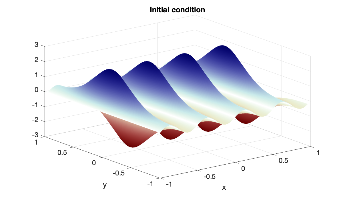

The following function computes the time derivative for the unknowns which have a vector shape. The actual calculations, however, take place using the matrix shape.

f13_2_heat.m

function du_dt = timederiv(t, u, p)
    [alpha, Dxx, Dyy, vec, unvec] = p{:};
    U = unvec(u);
    Uxx = Dxx * U;  Uyy = U * Dyy';     % 2nd partials
    dU_dt = alpha * (Uxx + Uyy);  % PDE
    du_dt = vec(dU_dt);
end

Since this problem is parabolic, a stiff time integrator is appropriate.

odefun = @(t, u) f13_2_heat(t, u, {0.1, Dxx, Dyy, vec, unvec});
sol = ode15s(odefun, [0, 0.2], vec(U0));
sol = solutionFcn(ivp, 0, 0.2);
U = @(t) unvec(deval(sol, t));

Unrecognized function or variable 'ivp'.

We can use the function U defined above to get the solution at any time. Its output is a matrix of values on the grid.

Source

surf(X', Y', U(0.05)')
clim([-mx, mx]),  shading interp
colormap(redsblues)
xlabel('x'),  ylabel('y')  
title('Solution at t = 0.05')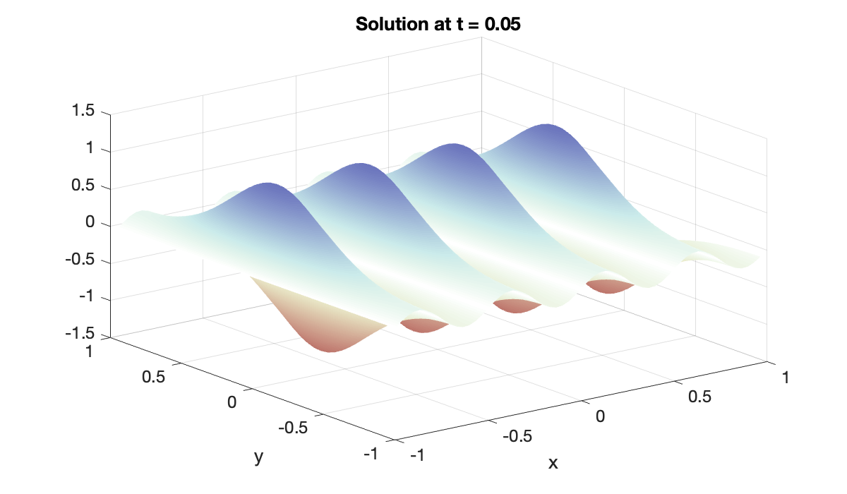

Array indices must be positive integers or logical values.

An animation shows convergence toward a uniform value.

Source

title('Heat equation on a periodic domain')
vid = VideoWriter("figures/2d-heat.mp4","MPEG-4");
vid.Quality = 85;
open(vid);
for t = linspace(0, 0.2, 61)
    cla, surf(X', Y', U(t)')
    zlim([-3, 3]),  clim([-mx, mx])
    shading interp
    str = sprintf("t = %.2f", t);
    text(-0.9, 0.75, 2, str, fontsize=14);
    writeVideo(vid, frame2im(getframe(gcf)));
end
close(vid)

Example 13.2.3

The first step is to define a discretization of the domain and the initial state.

m = 50;  n = 40;
[x, Dx, Dxx] = diffcheb(m, [-1, 1]);
[y, Dy, Dyy] = diffcheb(n, [-1, 1]);
[mtx, X, Y] = tensorgrid(x, y);
u_init = @(x, y) (1+y) .* (1-x).^4 .* (1+x).^2 .* (1-y.^4);

We define functions extend and chop to deal with the Dirichlet boundary conditions.

chop = @(U) U(2:m, 2:n);
z = zeros(1, n-1);
extend = @(W) [ zeros(m+1, 1) [z; W; z] zeros(m+1, 1)];

Now we define the pack and unpack functions, using another call to Algorithm 13.2.1 to get reshaping functions for the interior points.

[~, ~, ~, vec, unvec] = tensorgrid(x(2:m), y(2:n));
pack = @(U) vec(chop(U));
unpack = @(w) extend(unvec(w));

Now we can define and solve the IVP using a stiff solver.

f13_2_advdiff.m

function du_dt = timederiv(t, u, p)
    [ep, Dx, Dxx, Dy, Dyy, pack, unpack] = p{:};
    U = unpack(u);
    Uxx = Dxx * U;  Uyy = U * Dyy'; 
    dU_dt = 1 - Dx * U + ep * (Uxx + Uyy);  % PDE
    du_dt = pack(dU_dt);
end

odefun = @(t, u) f13_2_advdiff(t, u, {0.05, Dx, Dxx, Dy, Dyy, pack, unpack});
u_init = pack(mtx(u_init));
sol = ode15s(odefun, [0, 2], u_init);

When we evaluate the solution at a particular value of $t$ , we get a vector of the interior grid values. The unpack converts this to a complete matrix of grid values.

U = @(t) unpack(deval(sol, t));

clf,  pcolor(X', Y', U(0.5)')
clim([0, 2.3]), shading interp
axis equal,  colormap(sky), colorbar
title('Advection-diffusion at t = 0.5')  
xlabel('x'),  ylabel('y')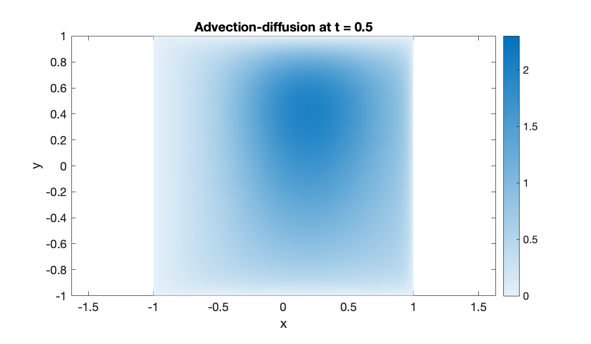

Source

hold on
vid = VideoWriter("figures/2d-advdiff.mp4","MPEG-4");
vid.Quality = 85;
open(vid);
title("Advection-diffusion in 2d")
for t = linspace(0, 2, 81)
    cla, pcolor(X', Y', U(t)')
    shading interp
    str = sprintf("t = %.2f", t);
    text(-1.5, 0.75, str, fontsize=14);
    writeVideo(vid, frame2im(getframe(gcf)));
end
close(vid)

Example 13.2.4

We start with the discretization and initial condition.

m = 40; n = 42;
[x, Dx, Dxx] = diffcheb(m, [-2, 2]);
[y, Dy, Dyy] = diffcheb(n, [-2, 2]);
[mtx, X, Y] = tensorgrid(x, y);

u_init = @(x, y) (x+0.2) .* exp(-12*(x.^2 + y.^2));
U0 = mtx(u_init);
V0 = zeros(size(U0));

We need to define chopping and extension for the $u$ component. This looks the same as in Example 13.2.3.

chop = @(U) U(2:m, 2:n);
z = zeros(1, n-1);
extend = @(U) [ zeros(m+1, 1) [z; U; z] zeros(m+1, 1)];

The vec and unvec operations are different for the interior-only grid and the full grid.

[~, ~, ~, vec_v, unvec_v] = tensorgrid(x, y);
[~, ~, ~, vec_u, unvec_u] = tensorgrid(x(2:m), y(2:n));
N = (m-1) * (n-1);

pack = @(U, V) [vec_u(chop(U)); vec_v(V)];
unpack = @(u) f13_2_wave_unpack(u, N, unvec_u, unvec_v, extend);

f13_2_wave_unpack.m

function [U, V] = unpack(w, N, unvec_u, unvec_v, extend)
    U = extend( unvec_u(w(1:N)) );
    V = unvec_v(w(N+1:end));
end

We can now define and solve the IVP. Since this problem is hyperbolic, a nonstiff integrator is faster than a stiff one.

f13_2_wave.m

function dw_dt = timederiv(t, w, p)
    [Dxx, Dyy, pack, unpack] = p{:};
    [U, V] = unpack(w);
    dU_dt = V;
    dV_dt = Dxx * U + U * Dyy';
    dw_dt = pack(dU_dt, dV_dt);
end

odefun = @(t, u) f13_2_wave(t, u, {Dxx, Dyy, pack, unpack});
ivp.InitialTime = 0;
z_init = pack(U0, V0);
ivp_sol = ode45(odefun, [0, 4], z_init);
sol = @(t) deval(ivp_sol, t);

clf
[U, V] = unpack(sol(0.5));
pcolor(X', Y', U')
axis equal,  clim([-0.1, 0.1])
colormap(redsblues),  shading interp
xlabel("x"),  ylabel("y")
title("Wave equation at t = 0.5")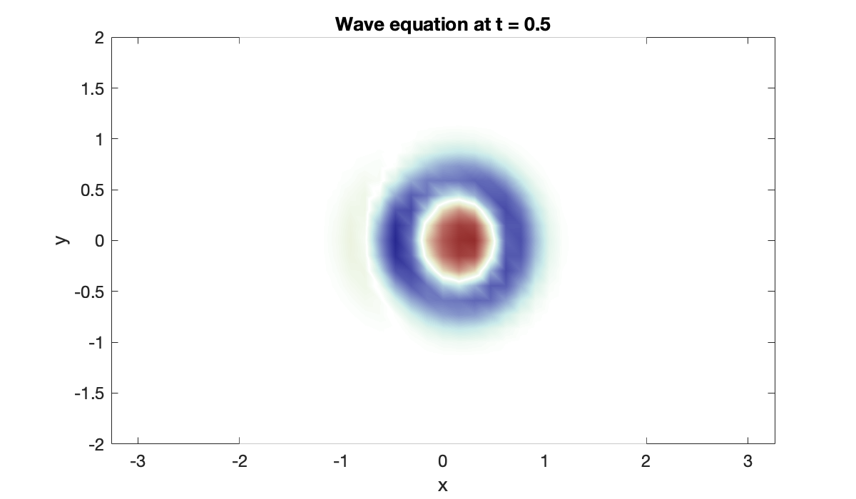

Source

hold on
vid = VideoWriter("figures/2d-wave.mp4","MPEG-4");
vid.Quality = 85;
open(vid);
title("Wave equation in 2d")
for t = linspace(0, 4, 121)
    [U, V] = unpack(sol(t));
    cla, pcolor(X, Y, U)
    shading interp
    str = sprintf("t = %.2f", t);
    text(-3, 1.75, str, fontsize=14);
    writeVideo(vid, frame2im(getframe(gcf)));
end
close(vid)

13.3 Laplace and Poisson equations¶

Example 13.3.1

A = [1, 2; -2, 0];
B = [1, 10, 100; -5, 5, 3];
disp("A:")
disp(A)
disp("B:")
disp(B)

A:

     1     2
    -2     0

B:

     1    10   100
    -5     5     3

Applying the definition manually, we get

A_kron_B = [
    A(1,1)*B  A(1,2)*B;
    A(2,1)*B  A(2,2)*B
    ]

But it makes more sense to use kron.

kron(A, B)

Example 13.3.2

We make a crude discretization for illustrative purposes.

m = 6;  n = 5;
[x, Dx, Dxx] = diffmat2(m, [0, 3]);
[y, Dy, Dyy] = diffmat2(n, [-1, 1]);
[mtx, X, Y, vec, unvec, is_boundary] = tensorgrid(x, y);

Here is a look at the matrix we called $\mathbf{L}$ (the discrete Laplacian), before any modifications are made for the boundary conditions. The combination of Kronecker products and finite differences produces a characteristic sparsity pattern.

A = kron(speye(n+1), sparse(Dxx)) + kron(sparse(Dyy), speye(m+1));
clf,  spy(A)
title("System matrix before boundary conditions")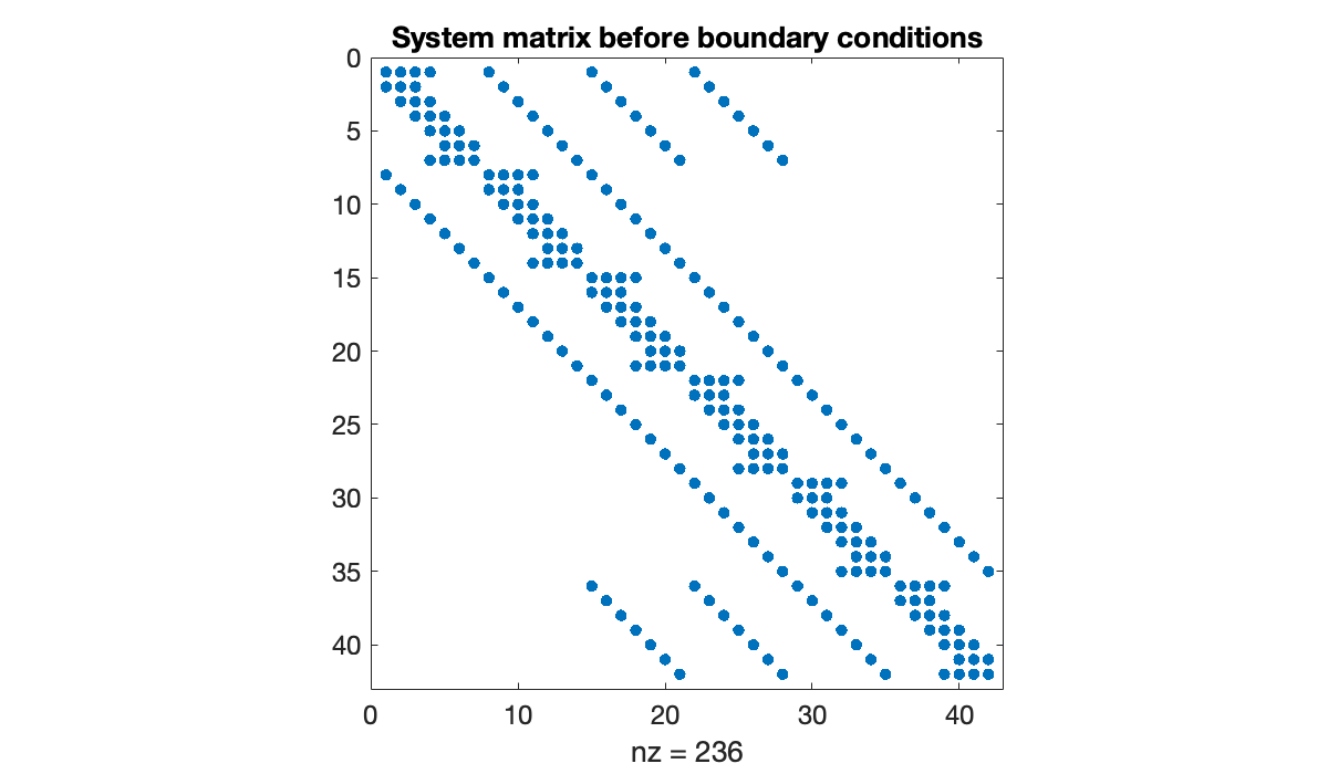

The number of equations is equal to $(m+1)(n+1)$ , which is the total number of points on the grid.

N = (m+1) * (n+1)

We now use the final output from Algorithm 13.2.1, which is a Boolean array indicating where the boundary points lie in the grid.

spy(is_boundary)
title("Boundary points")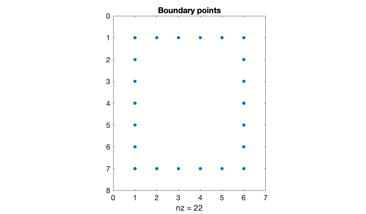

In order to impose Dirichlet boundary conditions, we use the boundary indicator to index into the rows of the system.

I = speye(N);
idx = vec(is_boundary);
A(idx, :) = I(idx, :);

spy(A)
title("System matrix with boundary conditions")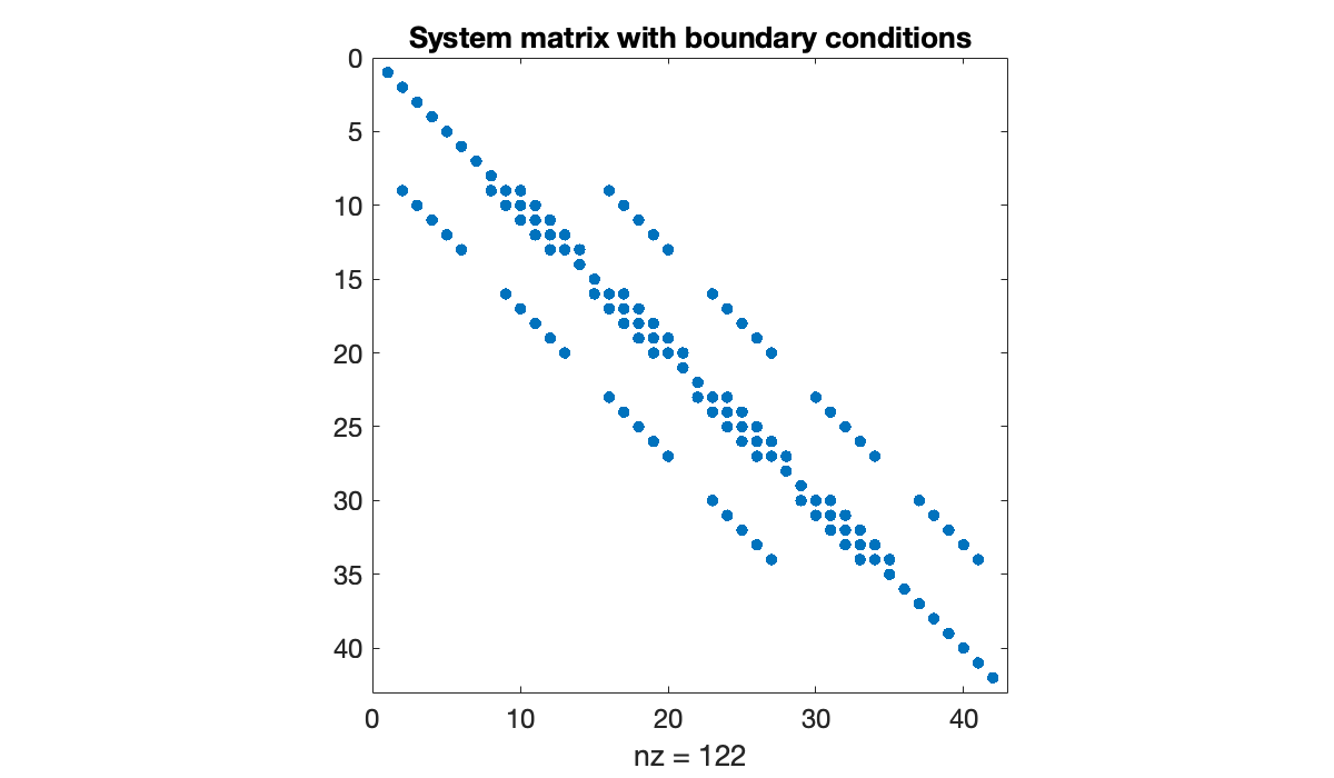

Next, we evaluate ϕ on the grid to get the forcing vector of the linear system, and then modify the boundary rows to hold the boundary values—in this case, zero.

phi = @(x, y) x.^2 - y + 2;
b = vec(mtx(phi));
b(idx) = 0;

Now we can solve the linear system $\mathbf{A}\mathbf{u}=\mathbf{b}$ for $\mathbf{u}$ and reinterpret it as the matrix-shaped $\mathbf{U}$ , the solution on our grid.

u = A \ b;
U = unvec(u)

Example 13.3.3

First we define the problem on $[0,1]\times[0,2]$ .

f = @(x, y) -sin(3*x .* y - 4*y) .* (9*y.^2 + (3*x - 4).^2);
g = @(x, y) sin(3*x .* y - 4*y);
xspan = [0, 1];
yspan = [0, 2];

Here is the finite-difference solution.

[X, Y, U] = poissonfd(f, g, 40, xspan, 60, yspan);

clf, surf(X', Y', U')
colormap(parula),  shading interp
colorbar
title("Solution of Poisson's equation")
xlabel("x"),  ylabel("y"),  zlabel("u(x,y)")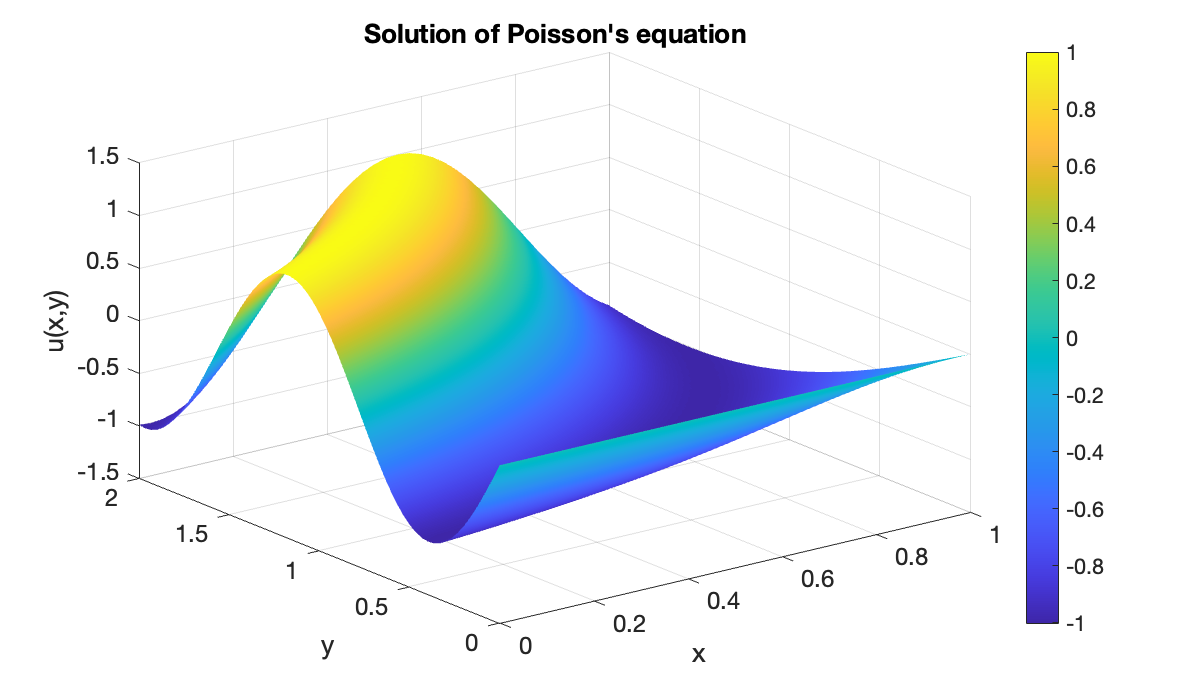

Since this is an artificial problem with a known solution, we can plot the error, which is a smooth function of $x$ and $y$ . It must be zero on the boundary; otherwise, we have implemented boundary conditions incorrectly.

err = g(X, Y) - U;
mx = max(abs(vec(err)));
pcolor(X', Y', err')
colormap(redsblues),  shading interp
clim([-mx, mx]),  colorbar
axis equal,  xlabel("x"),  ylabel("y")
title("Error")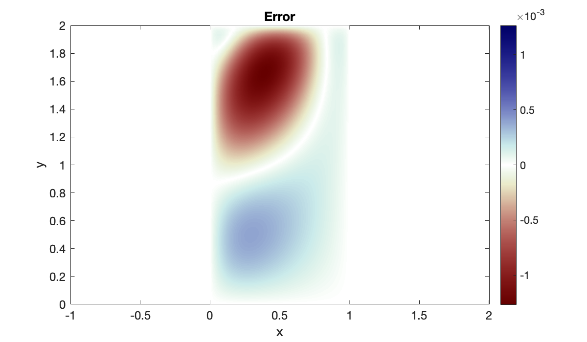

13.4 Nonlinear elliptic PDEs¶

Example 13.4.2

All we need to define are ϕ from (13.4.2) for the PDE, and a trivial zero function for the boundary condition.

lambda = 1.5;
phi = @(X, Y, U, Ux, Uxx, Uy, Uyy) Uxx + Uyy - lambda ./ (U + 1).^2;
g = @(x, y) zeros(size(x));

Here is the solution for $m=15$ , $n=8$ .

u = elliptic(phi, g, 15, [0, 2.5], 8, [0, 1]);
disp(sprintf("solution at (2, 0.6) is %.7f", u(2, 0.6)))

solution at (2, 0.6) is -0.2264594

Source

x = linspace(0, 2.5, 91);
y = linspace(0, 1, 51);
[mtx, X, Y] = tensorgrid(x, y);
clf,  pcolor(x, y, mtx(u)')
colormap(flipud(sky)),  shading interp,  colorbar
axis equal
xlabel("x"),  ylabel("y")
title("Deflection of a MEMS membrane")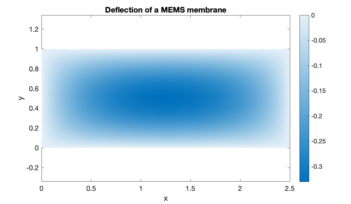

In the absence of an exact solution, how can we be confident that the solution is accurate? First, the Levenberg iteration converged without issuing a warning, so we should feel confident that the discrete equations were solved. Assuming that we encoded the PDE correctly, the remaining source of error is truncation from the discretization. We can estimate that by refining the grid a bit and seeing how much the numerical solution changes.

x_test = linspace(0, 2.5, 6);
y_test = linspace(0, 1 , 5);
mtx_test = tensorgrid(x_test, y_test);
format long
mtx_test(u)

u = elliptic(phi, g, 25, [0, 2.5], 14, [0, 1]);
mtx_test(u)

The original solution seems to be accurate to about four digits.

Example 13.4.3

phi = @(X, Y, U, Ux, Uxx, Uy, Uyy) 1 - Ux - 2*Uy + 0.05*(Uxx + Uyy);
g = @(x, y) zeros(size(x));
u = elliptic(phi, g, 32, [-1, 1], 32, [-1, 1]);

Source

x = linspace(-1, 1, 80);
y = x;
mtx = tensorgrid(x, y);
clf,  pcolor(x, y, mtx(u)')
colormap(parula),  shading interp,  colorbar
axis equal,  xlabel("x"),  ylabel("y")
title("Steady advection–diffusion")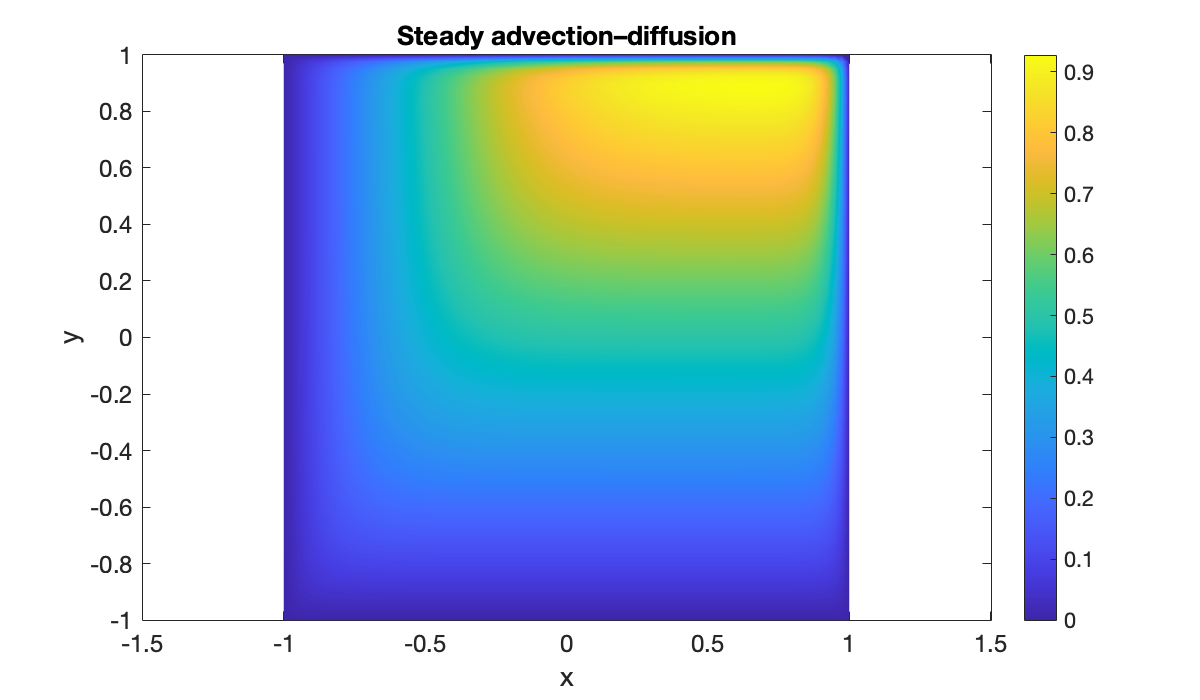

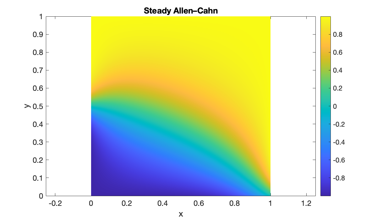
Example 13.4.4

The following defines the PDE and a nontrivial Dirichlet boundary condition for the square $[0,1]^2$ .

phi = @(X, Y, U, Ux, Uxx, Uy, Uyy) U .* (1-U.^2) + 0.05*(Uxx + Uyy);
g = @(x, y) tanh(5*(x + 2*y - 1));

We solve the PDE and then plot the result.

u = elliptic(phi, g, 36, [0, 1], 36, [0, 1]);

Source

x = linspace(0, 1, 80);
y = x;
mtx = tensorgrid(x, y);
clf,  pcolor(x, y, mtx(u)')
colormap(parula),  shading interp,  colorbar
axis equal,  xlabel("x"),  ylabel("y")
title("Steady Allen–Cahn")