As you learned when starting double integration in vector calculus, the simplest extension of an interval to two dimensions is a rectangle. We will use a particular notation for rectangles.
The idea of the tensor product is that each variable independently varies over a fixed set. When the interval is the same in each dimension, we may write .
The discretization of a two-dimensional tensor-product domain is straightforward.
Figure 13.1.1 shows a tensor-product grid on a rectangle. The grid is constructed from discretizations of with and with . Each grid point lies at the intersection of a vertical line through and a horizontal line through .
Figure 13.1.1:A tensor-product grid (dark gray) on a rectangle constructed from discretizations of with (blue) and with (red).
13.1.1Functions on grids
The double indexing of the grid set (13.1.3) implies an irresistible connection to matrices. Corresponding to any function defined on the rectangle is an matrix defined by collecting the values of at the points in the grid. This transformation of a function to a matrix is so important that we give it a formal name
13.1.2Parameterized surfaces
We are not limited to rectangles by tensor products. Many regions and surfaces may be parameterized by means of , , and , where and lie in a rectangle. Such “logically rectangular” surfaces include the unit disk,
and the unit sphere,
Example 13.1.3
For a function given in polar form, such as , construction of a function over the unit disk is straightforward using a grid in space.
r = range(0, 1, 41)
θ = range(0, 2π, 81)
F = [1 - r^4 for r in r, θ in θ]
plot(r, θ, F';
    legend=:none,
    color=:viridis,  fill=true,
    xlabel="r",  ylabel="θ",
title="A polar function")Of course, we are used to seeing such plots over the plane, not the plane.
In such functions the values along the line must be identical, and the values on the line should be identical to those on . Otherwise the interpretation of the domain as the unit disk is nonsensical. If the function is defined in terms of and , then those can be defined in terms of and using (13.1.5).
Example 13.1.3
For a function given in polar form, such as , construction of a function over the unit disk is straightforward using a grid in space.
r = linspace(0, 1, 41);
theta = linspace(0, 2*pi, 121);
[mtx, R, Theta] = tensorgrid(r, theta);
F = mtx(@(r, theta) 1 - r.^4);
clf,  colormap(parula)
contourf(R', Theta', F', 20)
shading flat
xlabel("r"),  ylabel("\theta"),
title("A polar function")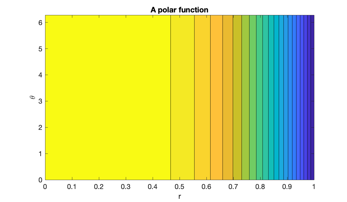
Of course, we are used to seeing such plots over the plane, not the plane. For this we create matrices for the coordinate functions and .
X = R .* cos(Theta);  Y = R .* sin(Theta);
contourf(X', Y', F', 20)
axis equal,  shading interp
xlabel('x'),  ylabel('y')
title('Function over the unit disk')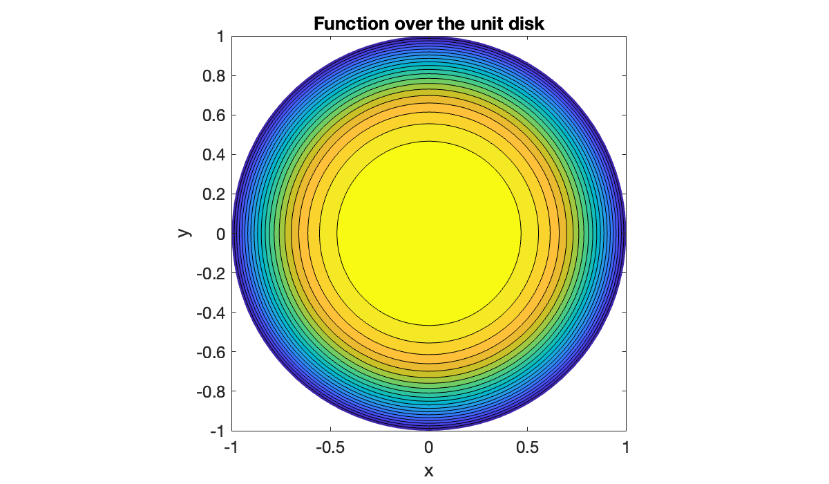
In such functions the values along the line must be identical, and the values on the line should be identical to those on . Otherwise the interpretation of the domain as the unit disk is nonsensical. If the function is defined in terms of and , then those can be defined in terms of and using (13.1.5).
Example 13.1.3
For a function given in polar form, such as , construction of a function over the unit disk is straightforward using a grid in space.
r = linspace(0, 1, 41)
theta = linspace(0, 2*pi, 121)
mtx, R, Theta, _, _, _ = FNC.tensorgrid(r, theta)

F = mtx(lambda r, theta: 1 - r**4)

contourf(R.T, Theta.T, F.T, levels=20)
colorbar()
xlabel("$r$"),  ylabel("$\\theta$");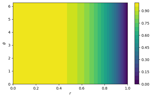
Of course, we are used to seeing such plots over the plane, not the plane. For this we create matrices for the coordinate functions and .
X, Y = R * cos(Theta), R * sin(Theta)
contourf(X.T, Y.T, F.T, levels=20)
colorbar(),  axis("equal")
xlabel("$x$"),  ylabel("$y$");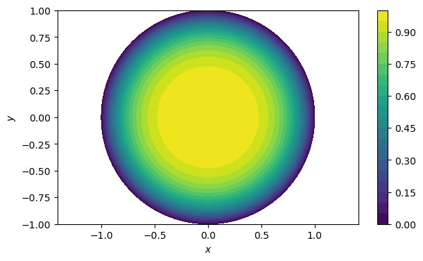
In such functions the values along the line must be identical, and the values on the line should be identical to those on . Otherwise the interpretation of the domain as the unit disk is nonsensical. If the function is defined in terms of and , then those can be defined in terms of and using (13.1.5).
13.1.3Partial derivatives
In order to solve boundary-value problems in one dimension by collocation, we replaced an unknown function by a vector of its values at selected nodes and discretized the derivatives in the equation using differentiation matrices. We use the same ideas in the 2D case: we represent a function by its values on a grid, and multiplication by differentiation matrices to construct discrete analogs of the partial derivatives and .
Consider first . In the definition of this partial derivative, the independent variable is held constant. Note that is constant within each column of . Thus, we may regard a single column as a discretized function of and, as usual, left-multiply by a differentiation matrix such as (10.3.6). We need to do this for each column of by , which is accomplished by . Altogether,
This relation is not an equality, because the left-hand side is a discretization of the exact partial derivative, while the right-hand side is a finite-difference approximation. Yet it is a natural analog for partial differentiation when we are given not but only the grid value matrix
Now we tackle . Here the inactive coordinate is held fixed within each row of . However, if we transpose , then the roles of rows and columns are swapped, and now varies independently down each column. This is analogous to the situation for the -derivative, so we left-multiply by a finite-difference matrix , and then transpose the entire result to restore the roles of and in the grid. Fortunately, linear algebra allows us to express the sequence transpose–left-multiply–transpose more compactly:
Keep in mind that the differentiation matrix is based on the discretization , and as such it must be . On the other hand, is based on and is . This is exactly what is needed dimensionally to make the products in (13.1.7) and (13.1.8) consistent. More subtly, if the differentiation is based on equispaced grids in each variable, the value of in a formula such as (5.4.5) will be different for and .
Example 13.1.4
We define a function and, for reference, its two exact partial derivatives.
u = (x, y) -> sin(π * x * y - y);
∂u_∂x = (x, y) -> π * y * cos(π * x * y - y);
∂u_∂y = (x, y) -> (π * x - 1) * cos(π * x * y - y);
We use an equispaced grid and second-order finite differences as implemented by diffmat2.
m, n = 80, 70;
x, Dx, _ = FNC.diffmat2(m, [0, 2]);
y, Dy, _ = FNC.diffmat2(n, [1, 3]);
mtx = (f, x, y) -> [f(x, y) for x in x, y in y];
Here is how the exact first partial derivatives look on the grid.
plot(layout=(1, 2), aspect_ratio=1, xlabel="x", ylabel="y")
contour!(x, y, mtx(∂u_∂x, x, y)';
    levels=12, colormap=:viridis, subplot=1, title="∂u/∂x")
contour!(x, y, mtx(∂u_∂y, x, y)';
levels=12, colormap=:viridis, subplot=2, title="∂u/∂y")Next, we compute the finite-difference approximations of these derivatives on the grid.
U = mtx(u, x, y)
∂xU = Dx * U
∂yU = U * Dy';
Finally, we compare the finite-difference approximations to the exact values, using a colormap that is symmetric about zero.
err_x = mtx(∂u_∂x, x, y) - ∂xU
err_y = mtx(∂u_∂y, x, y) - ∂yU

plot(layout=(1, 2), aspect_ratio=1,
    xlabel="x", ylabel="y")
M = maximum(abs, err_x)
contour!(x, y, err_x';
    levels=15, clims=(-M, M), colormap=:redsblues, fill=true,
    l=false, subplot=1, title="∂u/∂x error")
M = maximum(abs, err_y)
contour!(x, y, err_y';
    levels=15, clims=(-M, M), colormap=:redsblues, fill=true,
l=false, subplot=2, title="∂u/∂y error")Not surprisingly, the errors are largest where the derivatives themselves are largest.
Example 13.1.4
We define a function and, for reference, its two exact partial derivatives.
u = @(x, y) sin(pi * x .* y - y);
du_dx = @(x, y) pi * y .* cos(pi * x .* y - y);
du_dy = @(x, y) (pi * x - 1) .* cos(pi * x .* y - y);
We will use an equispaced grid and second-order finite differences as implemented by diffmat2.
m = 80;  [x, Dx] = diffmat2(m, [0, 2]);
n = 70;  [y, Dy] = diffmat2(n, [1, 3]);
[mtx, X, Y] = tensorgrid(x, y);
U = mtx(u);
dU_dX = mtx(du_dx);
dU_dY = mtx(du_dy);
First, we have a look at a plots of the exact partial derivatives.
clf,  subplot(1, 2, 1)
pcolor(X', Y', dU_dX')
axis equal,  shading interp
title('∂u/∂x')
subplot(1, 2, 2)
pcolor(X', Y', dU_dY')
axis equal,  shading interp
title('∂u/∂y')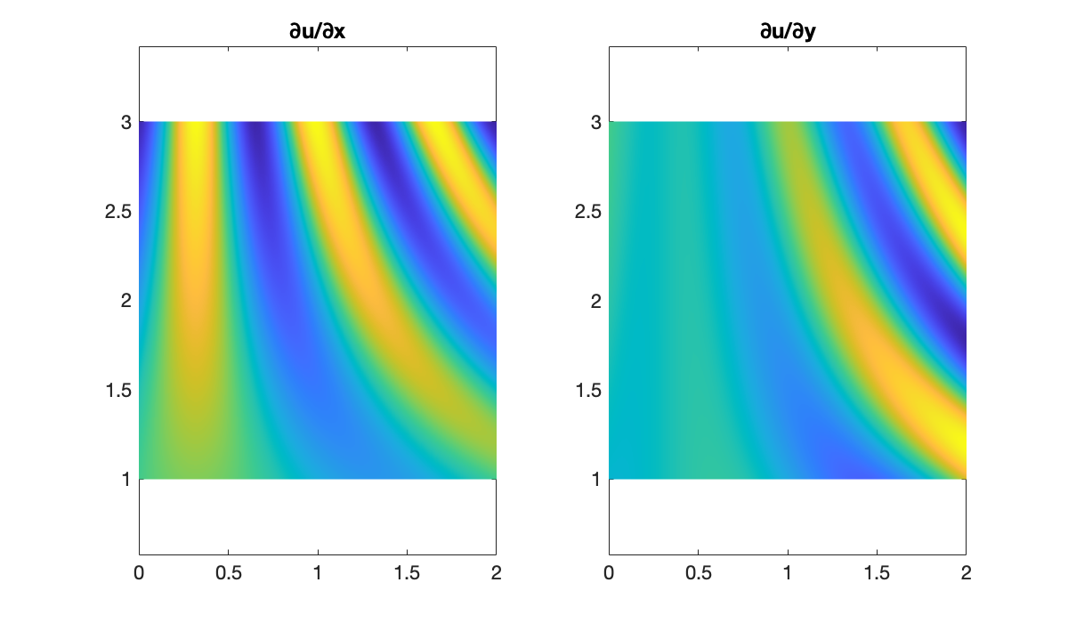
Now we compare the exact partial derivatives with their finite-difference approximations. Since these are signed errors, we use a colormap that is symmetric around zero.
err = dU_dX - Dx * U;
subplot(1, 2, 1)
M = max(abs(err(:)));
pcolor(X', Y', err')
colorbar,  clim([-M, M])
axis equal,  shading interp
title('error in ∂u/∂x')

err = dU_dY - U * Dy';
subplot(1,2,2)
M = max(abs(err(:)));
pcolor(X', Y', err')
colorbar,  clim([-M, M])
axis equal,  shading interp
colormap(redsblues)
title('error in ∂u/∂y')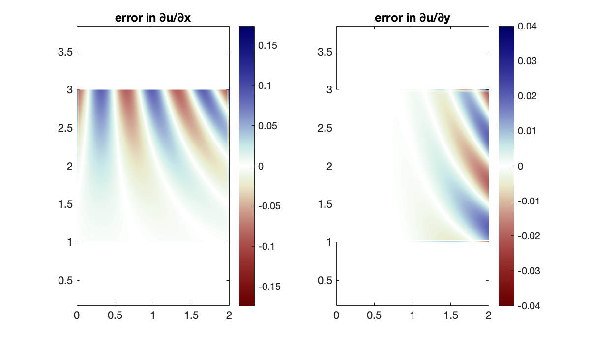
Not surprisingly, the errors are largest where the derivatives themselves are largest.
Example 13.1.4
We define a function and, for reference, its two exact partial derivatives.
u = lambda x, y: sin(pi * x * y - y)
du_dx = lambda x, y: pi * y * cos(pi * x * y - y)
du_dy = lambda x, y: (pi * x - 1) * cos(pi * x * y - y)
We will use an equispaced grid and second-order finite differences as implemented by diffmat2. First, we have a look at a plots of the exact partial derivatives.
m, n = 80, 70
x, Dx, Dxx = FNC.diffmat2(m, [0, 2])
y, Dy, Dyy = FNC.diffmat2(n, [1, 3])
mtx, X, Y, _, _, _ = FNC.tensorgrid(x, y)

U = mtx(u)
dU_dX = mtx(du_dx)
dU_dY = mtx(du_dy)

subplot(1, 2, 1)
contourf(X, Y, dU_dX)
title("$u$"),  axis("equal")
subplot(1, 2, 2)
contourf(X, Y, dU_dY)
title("$\\partial u/\\partial y$"),  axis("equal");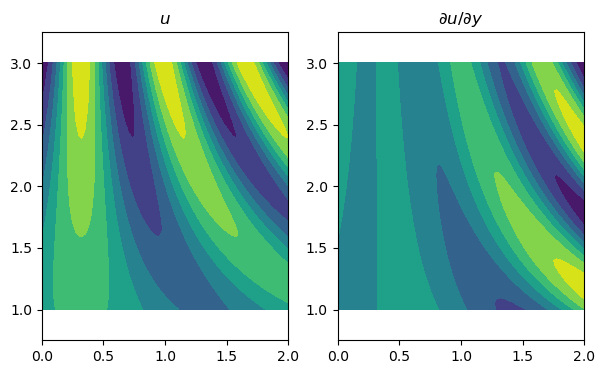
Now we compare the exact partial derivatives with their finite-difference approximations. Since these are signed errors, we use a colormap that is symmetric around zero.
subplot(1, 2, 1)
err_x = Dx @ U - dU_dX
M = max(abs(err_x))
pcolormesh(X, Y, err_x, shading="gouraud", cmap="RdBu", vmin=-M, vmax=M)
colorbar()
title("error in $\\partial u/\\partial x$"),  axis("equal")

subplot(1, 2, 2)
err_y = U @ Dy.T - dU_dY
M = max(abs(err_y))
pcolormesh(X, Y, err_y, shading="gouraud", cmap="RdBu", vmin=-M, vmax=M)
colorbar()
title("error in $\\partial u/\\partial y$"),  axis("equal");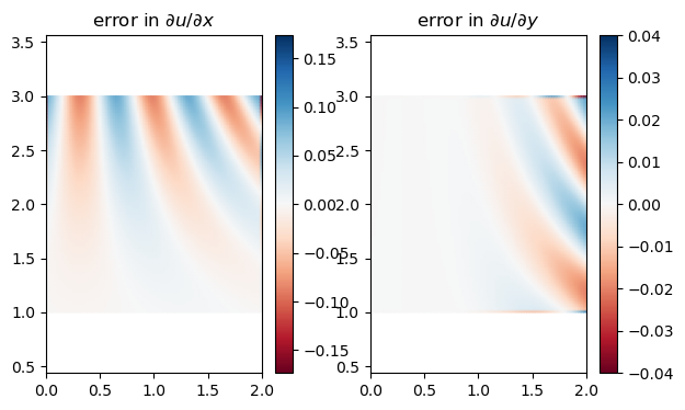
Not surprisingly, the errors are largest where the derivatives themselves are largest.
13.1.4Exercises
⌨ In each part, make side-by-side surface and contour plots of the given function over the given domain.
(a) ,
(b) ,
(c) ,
⌨ For each function in Exercise 13.1.1, make side-by-side surface plots of and using Chebyshev spectral differentiation.
⌨ For each function in Exercise 13.1.1, make a contour plot of the mixed derivative using Chebyshev spectral differentiation.
⌨ In each case, make a plot of the function given in polar or Cartesian coordinates over the unit disk.
(a)
(b)
(c)
⌨ Plot as a function on the unit sphere.
⌨ Plot as a function on the cylinder for .