Functions
Solution of least squares by the normal equations
1 2 3 4 5 6 7 8 9 10 11 12 13 14function x = lsnormal(A, b) % LSNORMAL Solve linear least squares by normal equations. % Input: % A coefficient matrix (m by n, m > n) % b right-hand side (m by 1) % Output: % x minimizer of || b - Ax || N = A' * A; z = A' * b; R = chol(N); w = forwardsub(R', z); % solve R'z=c x = backsub(R, w); % solve Rx=z end
Solution of least squares by QR factorization
1 2 3 4 5 6 7 8 9 10 11 12function x = lsqrfact(A, b) % LSQRFACT Solve linear least squares by QR factorization. % Input: % A coefficient matrix (m by n, m > n) % b right-hand side (m by 1) % Output: % x minimizer of || b - Ax || [Q, R] = qr(A, 0); % thin factorization c = Q' * b; x = backsub(R, c); end
QR factorization by Householder reflections
1 2 3 4 5 6 7 8 9 10 11 12 13 14 15 16 17 18 19 20 21 22 23 24 25 26 27 28function [Q,R] = qrfact(A) % QRFACT QR factorization by Householder reflections. % (demo only--not efficient) % Input: % A m-by-n matrix % Output: % Q, R Q m-by-m orthogonal, R m-by-n upper triangular such that A = QR [m, n] = size(A); Qt = eye(m); for k = 1:n z = A(k:m, k); w = [ -sign(z(1)) * norm(z) - z(1); -z(2:end) ]; nrmw = norm(w); if nrmw < eps, continue, end % nothing is done in this iteration v = w / nrmw; % removes v'*v in other formulas % Apply the reflection to each relevant column of A and Q for j = 1:n A(k:m, j) = A(k:m, j) - v * (2 * (v' * A(k:m, j))); end for j = 1:m Qt(k:m, j) = Qt(k:m, j) - v * (2 * (v' * Qt(k:m, j))); end end Q = Qt'; R = triu(A); % enforce exact triangularity end
Examples
3.1 Fitting functions to data
Example 3.1.1
Here are 5-year averages of the worldwide temperature anomaly as compared to the 1951–1980 average (source: NASA).
year = (1955:5:2000)';
y = [ -0.0480; -0.0180; -0.0360; -0.0120; -0.0040;
    0.1180; 0.2100; 0.3320; 0.3340; 0.4560 ];
scatter(year, y), axis tight
xlabel('year')
ylabel(('anomaly ({\circ}C)'));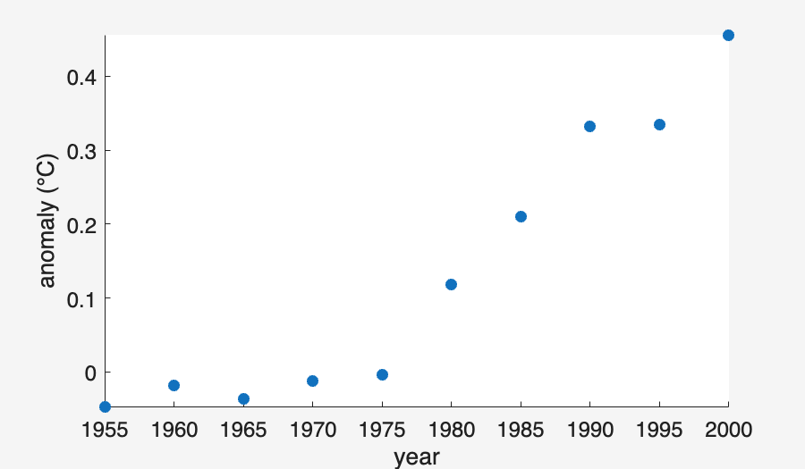
A polynomial interpolant can be used to fit the data. Here we build one using a Vandermonde matrix. First, though, we express time as decades since 1950, as it improves the condition number of the matrix.
t = (year - 1950) / 10;
n = length(t);
V = ones(n, 1);    % t^0
for j = 1:n-1
    V(:, j+1) = t .* V(:,j);
end
c = V \ y;    % solve for coefficients
We created the Vandermonde matrix columns in increasing-degree order. Thus, the coefficients in c also follow that ordering, which is the opposite of what MATLAB uses. We need to flip the coefficients before using them in polyval.
p = @(year) polyval(c(end:-1:1), (year - 1950) / 10);
hold on
fplot(p, [1955, 2000])    % plot the interpolating function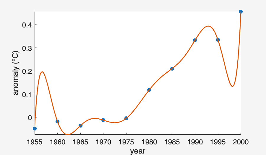
Example 3.1.2
Here are the 5-year temperature averages again.
year = (1955:5:2000)';
y = [ -0.0480; -0.0180; -0.0360; -0.0120; -0.0040;
    0.1180; 0.2100; 0.3320; 0.3340; 0.4560 ];
The standard best-fit line results from using a linear polynomial that meets the least-squares criterion.
Tip
Backslash solves overdetermined linear systems in a least-squares sense.
t = (year - 1950) / 10;    % better matrix conditioning later
V = [ t.^0 t ];            % Vandermonde-ish matrix
size(V)c = V \ y;
f = @(year) polyval(c(end:-1:1), (year - 1950) / 10);clf
scatter(year, y), axis tight
xlabel('year'), ylabel('anomaly ({\circ}C)')
hold on
fplot(f, [1955, 2000])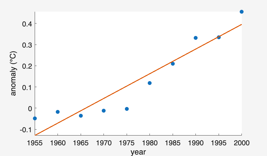
If we use a global cubic polynomial, the points are fit more closely.
V = [t.^0, t.^1, t.^2, t.^3]; % Vandermonde-ish matrix
size(V)Now we solve the new least-squares problem to redefine the fitting polynomial.
Tip
The definition of f above is in terms of c. When c is changed, then f has to be redefined.
c = V \ y;
f = @(year) polyval(c(end:-1:1), (year - 1950) / 10);
fplot(f, [1955, 2000])
legend('data', 'linear', 'cubic', 'Location', 'northwest');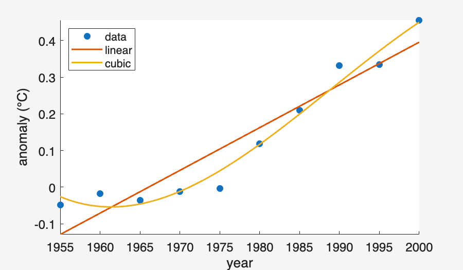
If we were to continue increasing the degree of the polynomial, the residual at the data points would get smaller, but overfitting would increase.
Example 3.1.3
k = (1:100)';
a = 1./k.^2;      % sequence
s = cumsum(a);    % cumulative summation
p = sqrt(6*s);
clf
plot(k, p, 'o-')
xlabel('k'), ylabel('p_k')
title('Sequence converging to \pi')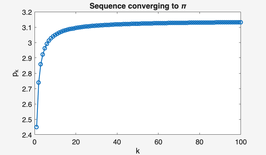
This graph suggests that maybe , but it’s far from clear how close the sequence gets. It’s more informative to plot the sequence of errors, . By plotting the error sequence on a log-log scale, we can see a nearly linear relationship.
ep = abs(pi - p);    % error sequence
loglog(k, ep, 'o')
title('Convergence')
xlabel('k'), ylabel('|p_k - \pi|'), axis tight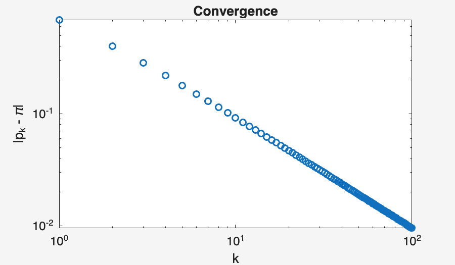
The straight line on the log-log scale suggests a power-law relationship where , or .
V = [ k.^0, log(k) ];    % fitting matrix
c = V \ log(ep) % coefficients of linear fitIn terms of the parameters and used above, we have
a = exp(c(1)), b = c(2)It’s tempting to conjecture that the slope asymptotically. Here is how the numerical fit compares to the original convergence curve.
hold on
loglog(k, a * k.^b)
legend('sequence', 'power-law fit');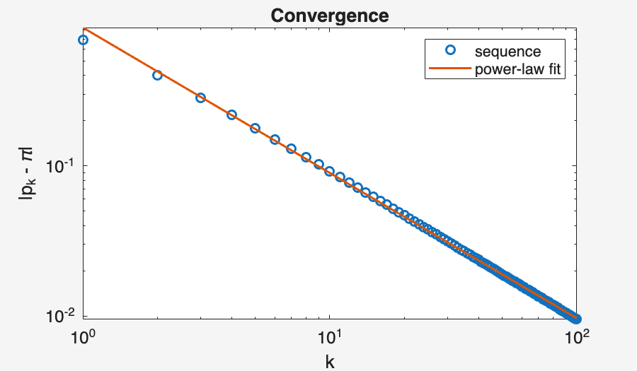
3.2 The normal equations
Example 3.2.1
Because the functions , , and 1 are linearly dependent, we should find that the following matrix is somewhat ill-conditioned.
Tip
The local variable scoping rule for loops applies to comprehensions as well.
t = linspace(0, 3, 400)';
A = [ sin(t).^2, cos((1+1e-7)*t).^2, t.^0 ];
kappa = cond(A)Now we set up an artificial linear least-squares problem with a known exact solution that actually makes the residual zero.
x = [1; 2; 1];
b = A * x;
Using backslash to find the least-squares solution, we get a relative error that is well below times machine epsilon.
x_BS = A \ b;
observed_err = norm(x_BS - x) / norm(x)
max_err = kappa * epsIf we formulate and solve via the normal equations, we get a much larger relative error. With , we may not be left with more than about 2 accurate digits.
N = A'*A;
x_NE = N\(A'*b);
observed_err = norm(x_NE - x) / norm(x)
digits = -log10(observed_err)3.3 The QR factorization
Example 3.3.1
MATLAB provides access to both the thin and full forms of the QR factorization.
A = magic(5);
A = A(:, 1:4);
[m, n] = size(A)Here is the full form:
[Q, R] = qr(A);
szQ = size(Q), szR = size(R)We can test that is an orthogonal matrix:
QTQ = Q' * Q
norm(QTQ - eye(m))With a second input argument given to qr, the thin form is returned. (This is usually the one we want in practice.)
[Q_hat, R_hat] = qr(A, 0);
szQ_hat = size(Q_hat), szR_hat = size(R_hat)Now cannot be an orthogonal matrix, because it is not square, but it is still ONC. Mathematically, is a identity matrix.
Q_hat' * Q_hat - eye(n)Example 3.3.2
We’ll repeat the experiment of Example 3.2.1, which exposed instability in the normal equations.
t = linspace(0, 3, 400)';
A = [ sin(t).^2, cos((1+1e-7)*t).^2, t.^0 ];
x = [1; 2; 1];
b = A * x;
The error in the solution by Function 3.3.2 is similar to the bound predicted by the condition number.
observed_error = norm(lsqrfact(A, b) - x) / norm(x)
error_bound = cond(A) * eps3.4 Computing QR factorizations
Example 3.4.1
We will use Householder reflections to produce a QR factorization of a matrix.
A = magic(6);
A = A(:, 1:4);
[m, n] = size(A)Our first step is to introduce zeros below the diagonal in column 1 by using (3.4.4) and (3.4.1).
z = A(:, 1);
v = z - norm(z) * eye(m,1);
P_1 = eye(m) - 2 / (v' * v) * (v * v');
We check that this reflector introduces zeros as it should:
P_1 * zNow we replace by .
A = P_1 * AWe are set to put zeros into column 2. We must not use row 1 in any way, lest it destroy the zeros we just introduced. So we leave it out of the next reflector.
z = A(2:m, 2);
v = z - norm(z) * eye(m-1, 1);
P_2 = eye(m-1) - 2 / (v' * v) * (v * v');
We now apply this reflector to rows 2 and below only.
A(2:m, 2:n) = P_2 * A(2:m, 2:n)We need to iterate the process for the last two columns.
for j = 3:n
    z = A(j:m,j);
    k = m-j+1;
    v = z - norm(z) * eye(k, 1);
    P = eye(k) - 2 / (v' * v) * (v * v');
    A(j:m, j:n) = P * A(j:m, j:n);
end
We have now reduced the original to an upper triangular matrix using four orthogonal Householder reflections:
R = A