When is meant to be time, sometimes we write (read “u-dot”) instead of .
Linear problems can be solved in terms of integrals. Defining the integrating factor , the solution is derived from
In many cases, however, the necessary integrals cannot be done in closed form. Some nonlinear ODEs, such as separable equations, may also be solvable with a short formula, perhaps with difficult integrations. Most often, though, there is no analytic formula available for the solution.
An ODE may have higher derivatives of the unknown solution present. For example, a second-order ordinary differential equation is often given in the form . A second-order IVP requires two conditions at the initial time in order to specify a solution completely. As we will see in IVP systems, we are always able to reformulate higher-order IVPs in a first-order form, so we will deal with first-order problems exclusively.
6.1.1Numerical solutions
6.1.2Existence and uniqueness
There are simple IVPs that do not have solutions at all possible times.
Example 6.1.3
The equation gives us some trouble.
f(u, p, t) = (t + u)^2
ivp = ODEProblem(f, 1.0, (0.0, 1.0))
sol = solve(ivp, Tsit5());
┌ Warning: At t=0.7853839417697202, dt was forced below floating point epsilon 1.1102230246251565e-16, and step error estimate = 42.16289878637392. Aborting. There is either an error in your model specification or the true solution is unstable (or the true solution can not be represented in the precision of Float64).
└ @ SciMLBase ~/.julia/packages/SciMLBase/4MHGc/src/integrator_interface.jl:671
The warning message we received can mean that there is a bug in the formulation of the problem. But if everything has been done correctly, it suggests that the solution may not exist past the indicated time. This is a possibility in nonlinear ODEs.
plot(sol, label="";
    xlabel=L"t",  yaxis=(:log10, L"u(t)"),
title="Finite-time blowup")Example 6.1.3
The equation gives us some trouble.
f = @(t, u) (t + u)^2;
u0 = 1;
tspan = [0, 1];
[t, u] = ode45(f, tspan, u0);
Warning: Failure at t=7.853789e-01. Unable to meet integration tolerances without reducing the step size below the smallest value allowed (1.776357e-15) at time t.The warning message we received can mean that there is a bug in the formulation of the problem. But if everything has been done correctly, it suggests that the solution simply may not exist past the indicated time. This is a possibility in nonlinear ODEs.
clf
semilogy(t, u)
xlabel("t")
ylabel("u(t)")
title(("Finite-time blowup"));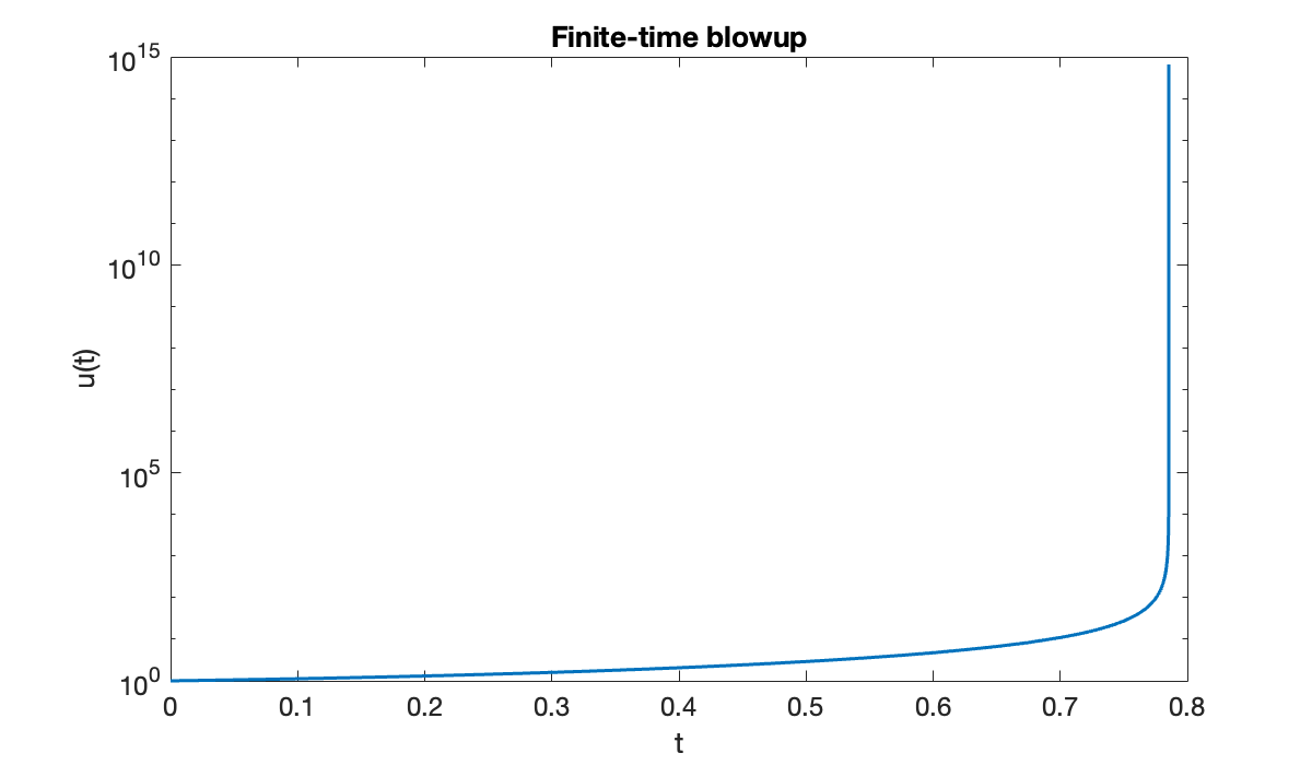
Example 6.1.3
The equation gives us some trouble.
Tip
It’s a good idea to check sol.success after calling solve_ivp. If it’s False, the solution may not be reliable.
f = lambda t, u: (t + u) ** 2
sol = solve_ivp(f, [0.0, 1.0], [1.0])
if not sol.success:
    print(sol.message)
Required step size is less than spacing between numbers.
The warning message we received can mean that there is a bug in the formulation of the problem. But if everything has been done correctly, it suggests that the solution may not exist past the indicated time. This is a possibility in nonlinear ODEs.
semilogy(sol.t, sol.y[0, :])
xlabel("$t$")
ylabel("$u(t)$")
title(("Blowup in finite time"));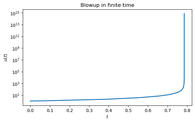
We can also produce an IVP that has more than one solution.
The functions and both satisfy the differential equation and the initial condition . Thus the corresponding IVP has more than one solution.
The following standard theorem gives us a condition that is easy to check and guarantees that a unique solution exists. But it is not the most general possible such condition, so there are problems with a unique solution that it cannot detect. We state the theorem without proof.
If the derivative exists and is bounded by a constant for all and all , then the initial-value problem (6.1.1) has a unique solution for .
6.1.3Conditioning of first-order IVPs
In a numerical context we have to be concerned about the conditioning of the IVP. There are two key items in (6.1.1) that we might consider to be the data of the initial-value ODE problem: the function , and the initial value . It’s easier to discuss perturbations to numbers than to functions, so we will focus on the effect of on the solution, using the following theorem that we give without proof. Happily, its conditions are identical to those in Theorem 6.1.1.
If the derivative exists and is bounded by a constant for all and all , then the solution of with initial condition satisfies
for all sufficiently small .
Numerical solutions of IVPs have errors, and those errors can be seen as perturbations to the solution. Theorem 6.1.2 gives an upper bound of on the infinity norm (i.e., pointwise) absolute condition number of the solution with respect to perturbations at an initial time. However, the upper bound may be a terrible overestimate of the actual sensitivity for a particular problem.
Example 6.1.5
Consider the ODEs and . In each case we compute , so the condition number bound from Theorem 6.1.2 is in both problems. However, they behave quite differently. In the case of exponential growth, , the bound is the actual condition number.
But with , solutions actually get closer together with time.
In this case the actual condition number is one, because the initial difference between solutions is the largest over all time. Hence the exponentially growing bound is a gross overestimate.
Example 6.1.5
Consider the ODEs and . In each case we compute , so the condition number bound from Theorem 6.1.2 is in both problems. However, they behave quite differently. In the case of exponential growth, , the bound is the actual condition number.
Source
clf
for u0 = [0.7, 1, 1.3]    % initial values
    fplot(@(t) exp(t) * u0, [0, 3]), hold on
end
xlabel('t')
ylabel('u(t)')
title(('Exponential divergence of solutions'));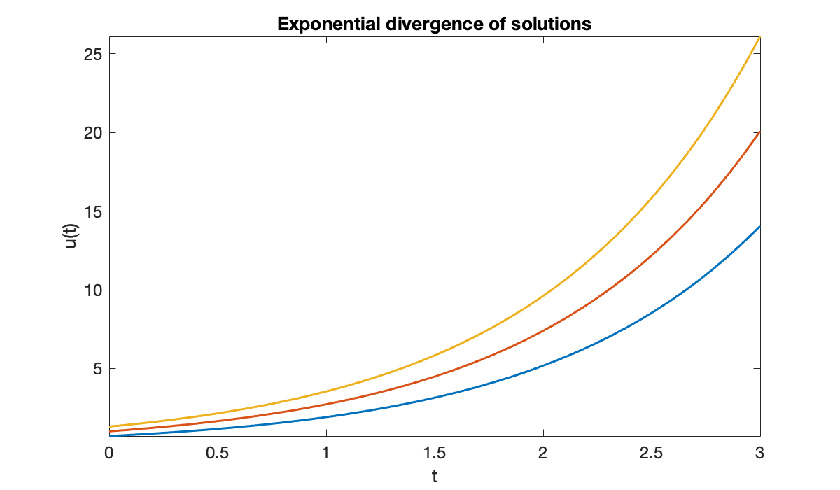
But with , solutions actually get closer together with time.
Source
clf
for u0 = [0.7, 1, 1.3]    % initial values
    fplot(@(t) exp(-t) * u0, [0, 3]), hold on
end
xlabel('t')
ylabel('u(t)')
title(('Exponential convergence of solutions'));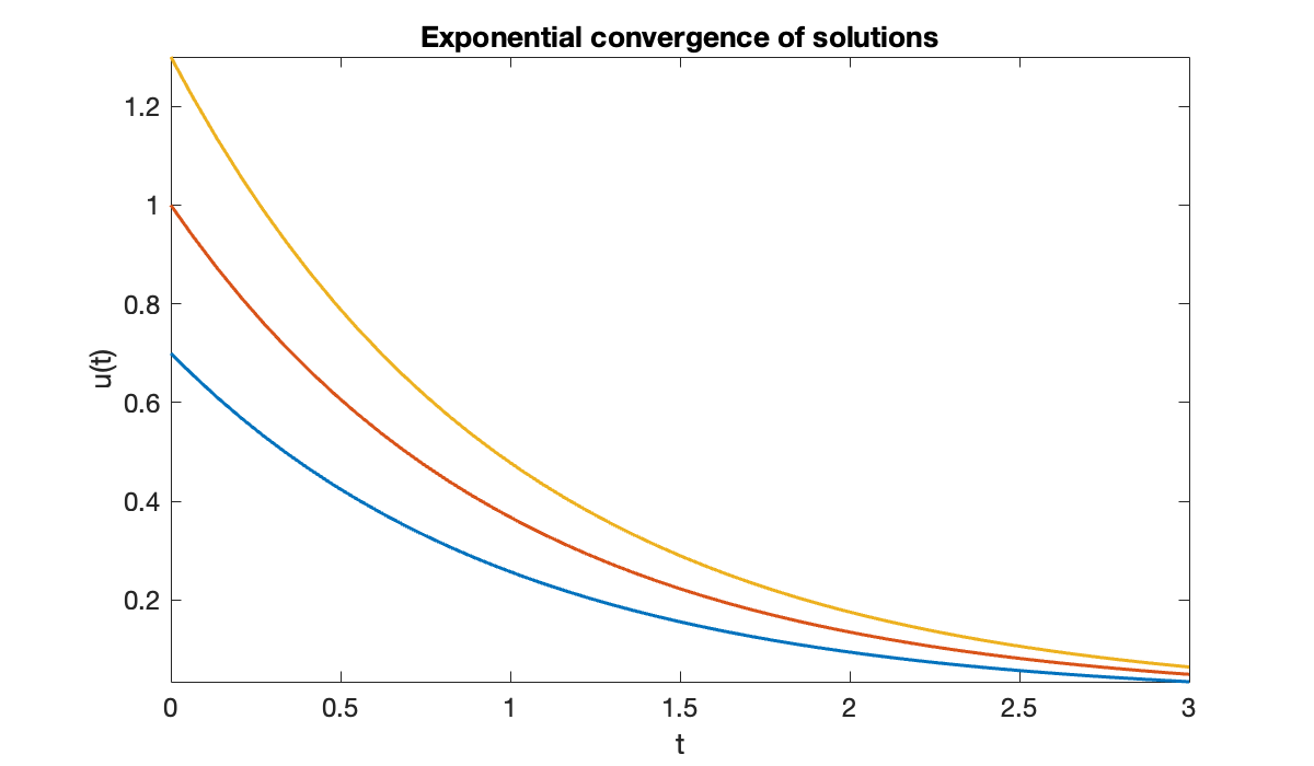
In this case the actual condition number is one, because the initial difference between solutions is the largest over all time. Hence the exponentially growing bound is a gross overestimate.
Example 6.1.5
Consider the ODEs and . In each case we compute , so the condition number bound from Theorem 6.1.2 is in both problems. However, they behave quite differently. In the case of exponential growth, , the bound is the actual condition number.
t = linspace(0, 3, 200)
u = array([exp(t) * u0 for u0 in [0.7, 1, 1.3]])
plot(t, u.T)
xlabel("$t$")
ylabel("$u(t)$")
title(("Exponential divergence of solutions"));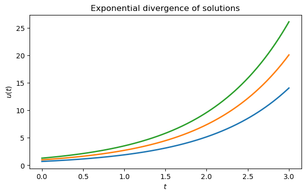
But with , solutions actually get closer together with time.
t = linspace(0, 3, 200)
u = array([exp(-t) * u0 for u0 in [0.7, 1, 1.3]])
plot(t, u.T)
xlabel("$t$")
ylabel("$u(t)$")
title(("Exponential convergence of solutions"));
In this case the actual condition number is one, because the initial difference between solutions is the largest over all time. Hence, the exponentially growing upper bound is a gross overestimate.
In general, solutions can diverge from, converge to, or oscillate around the original trajectory in response to perturbations. We won’t fully consider these behaviors and their implications for numerical methods again until a later chapter.
6.1.4Exercises
✍ For each IVP, determine whether the problem satisfies the conditions of Theorem 6.1.2. If so, determine the smallest possible value for .
(a)
(b)
(c)
(d)
⌨ For each ODE in the preceding problem, assume that is initially equal to 1 on the given interval. Solve the resulting IVP as in Example 6.1.2, and make a plot of the solution.
✍ Use an integrating factor to find the solution of each problem in analytic form.
(a)
(b)
✍ Consider the IVP , .
(a) Does Theorem 6.1.1 apply to this problem?
(b) Show that is a solution of the IVP.
(c) Does this solution necessarily exist for all ?
⌨ Using the method in Example 6.1.2, compute solutions to the logistic equation with harvesting,
with and , for the initial conditions , , , , , . Show all the solutions together on one plot with . (Note: One of the solutions will throw a warning and fail to reach , but you can plot it anyway.)
⌨ (a) Using the method in Example 6.1.2, solve the IVP , , for . Plot all the solutions on a single graph.
(b) All of the solutions in part (a) eventually settle into one of two periodic oscillations. To two digits of accuracy, find the value of in at which the selected long-term solution changes. (This will take repeated trials, narrowing down the range for each time.)
⌨ Experimental evidence (see Newton et al. (1981)) shows that a 300-mg oral dose of caffeine, such as might be found in a large mug of drip-brewed coffee, creates a concentration of about 8 /mL in blood plasma. This boost is followed by first-order kinetics with a half-life of about 6 hours (although this rate can vary a great deal from person to person). We can model the caffeine concentration due to one drink taken over half an hour via
where and
Solve the IVP and make a plot of the caffeine concentration for 12 hours. Then change (half-life of 8 hours) and plot the solution again.
⌨ A reasonable model of the velocity of a skydiver is
where is gravitational acceleration, is the mass of the skydiver with parachute, and quantifies the effect of air resistance. At the US Air Force Academy, a training jump starts at about 1200 m and has for and for . (This is an oversimplification; see Meade & Struthers (1999).)
(a) Solve the IVP for for an 80-kg cadet for , and plot the solution.
(b) The total distance fallen up to time is . Use Function 5.7.1 to calculate and plot the altitude of the cadet as a function of time.
(c) In part (b), you should have found that the altitude becomes negative. Use Function 4.4.1 to determine accurately when the cadet reaches the ground.
- Newton, R., Broughton, L. J., Lind, M. J., Morrison, P. J., Rogers, H. J., & Bradbrook, I. D. (1981). Plasma and Salivary Pharmacokinetics of Caffeine in Man. European Journal of Clinical Pharmacology, 21(1), 45–52. 10.1007/BF00609587
- Meade, D. B., & Struthers, A. A. (1999). Differential Equations in the New Millennium: The Parachute Problem. International Journal of Engineering Education, 15(6), 417–424.