Chapter 3

Here are 5-year averages of the worldwide temperature anomaly as compared to the 1951–1980 average (source: NASA).

year = arange(1955,2005,5)
y = array([ -0.0480, -0.0180, -0.0360, -0.0120, -0.0040,
    0.1180, 0.2100, 0.3320, 0.3340, 0.4560 ])

fig, ax = subplots()
ax.scatter(year, y, color="k", label="data")
xlabel("year")
ylabel("anomaly (degrees C)")
title("World temperature anomaly");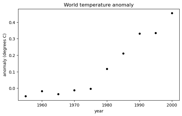

A polynomial interpolant can be used to fit the data. Here we build one using a Vandermonde matrix. First, though, we express time as decades since 1950, as it improves the condition number of the matrix.

from scipy import linalg
t = (year - 1950) / 10
V = vander(t)
c = linalg.solve(V, y)
print(c)

[ 1.03111111e-02 -2.54666667e-01  2.69480635e+00 -1.59628889e+01
  5.80155778e+01 -1.33273472e+02  1.91960567e+02 -1.65455972e+02
  7.63617381e+01 -1.41140000e+01]

The coefficients in vector c are used to create a polynomial. Then we create a function that evaluates the polynomial after changing the time variable as we did for the Vandermonde matrix.

p = poly1d(c)    # convert to a polynomial
tt = linspace(1955, 2000, 500)
ax.plot(tt, p((tt - 1950) / 10), label="interpolant")
ax.legend();
fig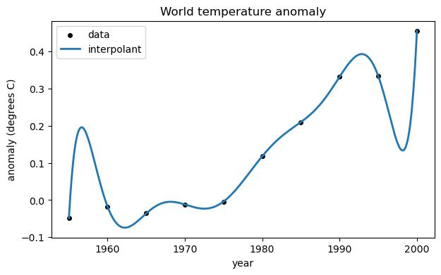

As you can see, the interpolant does represent the data, in a sense. However it’s a crazy-looking curve for the application. Trying too hard to reproduce all the data exactly is known as overfitting.

Here are the 5-year temperature averages again.

year = arange(1955, 2005, 5)
y = array([-0.0480, -0.0180, -0.0360, -0.0120, -0.0040,
    0.1180, 0.2100, 0.3320, 0.3340, 0.4560])
t = (year - 1950) / 10

The standard best-fit line results from using a linear polynomial that meets the least-squares criterion.

V = array([ [t[i], 1] for i in range(t.size) ])    # Vandermonde-ish matrix
print(V.shape)

(10, 2)

from scipy.linalg import lstsq
c, res, rank, sv = lstsq(V, y)
p = poly1d(c)
f = lambda year: p((year - 1950) / 10)

```{code-cell}
fig, ax = subplots()
ax.scatter(year, y, color="k", label="data")
yr = linspace(1955, 2000, 500)
ax.plot(yr, f(yr), label="linear fit")

xlabel("year")
ylabel("anomaly (degrees C)")
title("World temperature anomaly");
ax.legend();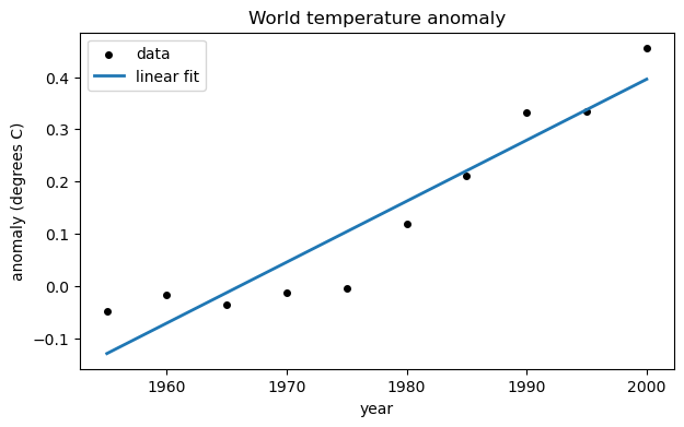

If we use a global cubic polynomial, the points are fit more closely.

V = array([ [t[i]**3,t[i]**2,t[i],1] for i in range(t.size) ])    # Vandermonde-ish matrix
print(V.shape)

(10, 4)

Now we solve the new least-squares problem to redefine the fitting polynomial.

c, res, rank, sv = lstsq(V, y)
yr = linspace(1955, 2000, 500)
ax.plot(yr, f(yr), label="cubic fit")
fig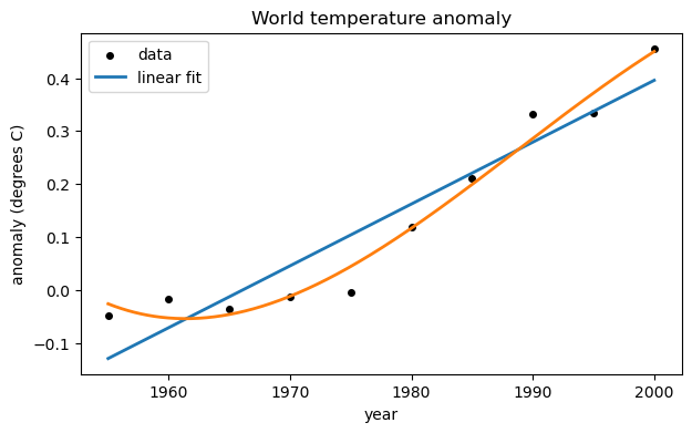

If we were to continue increasing the degree of the polynomial, the residual at the data points would get smaller, but overfitting would increase.

a = array([1 / (k+1)**2 for k in range(100)])
s = cumsum(a)        # cumulative summation
p = sqrt(6*s)

plot(range(100), p, "o")
xlabel("$k$") 
ylabel("$p_k$") 
title("Sequence convergence");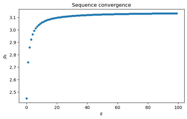

This graph suggests that maybe $p_k\to \pi$, but it’s far from clear how close the sequence gets. It’s more informative to plot the sequence of errors, $\epsilon_k= |\pi-p_k|$. By plotting the error sequence on a log-log scale, we can see a nearly linear relationship.

ep = abs(pi - p)    # error sequence
loglog(range(100), ep, "o")
xlabel("$k$") 
ylabel("error") 
title("Sequence convergence");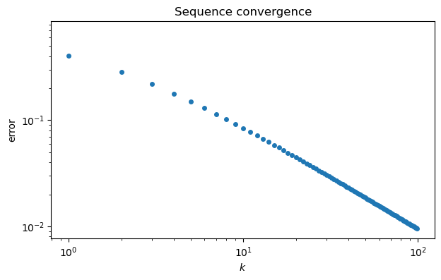

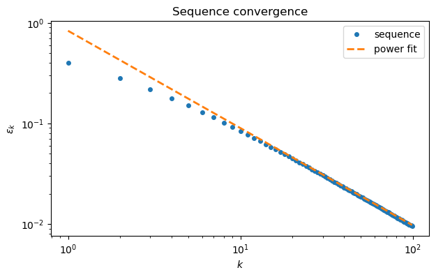
The straight line on the log-log scale suggests a power-law relationship where $\epsilon_k\approx a k^b$, or $\log \epsilon_k \approx b (\log k) + \log a$.

V = array([ [1, log(k+1)] for k in range(100) ])     # fitting matrix
c = lstsq(V, log(ep))[0]           # coefficients of linear fit
print(c)

[-0.18237525 -0.96741032]

In terms of the parameters $a$ and $b$ used above, we have

a, b = exp(c[0]), c[1]
print(f"b: {b:.3f}")

b: -0.967

It’s tempting to conjecture that the slope $b\to -1$ asymptotically. Here is how the numerical fit compares to the original convergence curve.

loglog(range(100), ep, "o", label="sequence")
k = arange(1,100)
plot(k, a*k**b, "--", label="power fit")
xlabel("$k$");  ylabel("error"); 
legend(); title("Sequence convergence");

Because the functions $\sin^2(t)$, $\cos^2(t)$, and 1 are linearly dependent, we should find that the following matrix is somewhat ill-conditioned.

from numpy.linalg import cond
t = linspace(0, 3, 400)
A = array([ [sin(t)**2, cos((1+1e-7)*t)**2, 1] for t in t ])
kappa = cond(A)
print(f"cond(A) is {kappa:.3e}")

cond(A) is 1.825e+07

Now we set up an artificial linear least-squares problem with a known exact solution that actually makes the residual zero.

x = array([1, 2, 1])
b = A @ x

Using backslash to find the least-squares solution, we get a relative error that is well below $\kappa$ times machine epsilon.

from scipy.linalg import lstsq
x_BS = lstsq(A, b)[0]
print(f"observed error: {norm(x_BS - x) / norm(x):.3e}")
print(f"conditioning bound: {kappa * finfo(float).eps:.3e}")

observed error: 2.019e-10
conditioning bound: 4.053e-09

If we formulate and solve via the normal equations, we get a much larger relative error. With $\kappa^2\approx 10^{14}$, we may not be left with more than about 2 accurate digits.

from scipy import linalg
N = A.T @ A
x_NE = linalg.solve(N, A.T @ b)
relative_err = norm(x_NE - x) / norm(x)
print(f"observed error: {relative_err:.3e}")
print(f"accurate digits: {-log10(relative_err):.2f}")

observed error: 5.991e-02
accurate digits: 1.22

NumPy provides access to both the thin and full forms of the QR factorization.

A = 1.0 + floor(9 * random.rand(6,4))
A.shape

Here is the full form:

from numpy.linalg import qr
Q, R = qr(A, "complete")
print(f"size of Q is {Q.shape}")
print("R:")
print(R)

size of Q is (6, 6)
R:
[[-13.7113092   -5.61580217 -10.72107688  -8.02257453]
 [  0.          -8.27422298  -6.25950658 -10.26643936]
 [  0.           0.          -5.3737406   -6.4622615 ]
 [  0.           0.           0.           3.387875  ]
 [  0.           0.           0.           0.        ]
 [  0.           0.           0.           0.        ]]

We can test that $\mathbf{Q}$ is an orthogonal matrix:

print(f"norm of (Q^T Q - I) is {norm(Q.T @ Q - eye(6)):.3e}")

norm of (Q^T Q - I) is 6.171e-16

The default for qr, and the one you usually want, is the thin form.

Q_hat, R_hat = qr(A)
print(f"size of Q_hat is {Q_hat.shape}")
print("R_hat:")
print(R_hat)

size of Q_hat is (6, 4)
R_hat:
[[-13.7113092   -5.61580217 -10.72107688  -8.02257453]
 [  0.          -8.27422298  -6.25950658 -10.26643936]
 [  0.           0.          -5.3737406   -6.4622615 ]
 [  0.           0.           0.           3.387875  ]]

Now $\hat{\mathbf{Q}}$ cannot be an orthogonal matrix, because it is not square, but it is still ONC. Mathematically, $\hat{\mathbf{Q}}^T \hat{\mathbf{Q}}$ is a $4\times 4$ identity matrix.

print(f"norm of (Q_hat^T Q_hat - I) is {norm(Q_hat.T @ Q_hat - eye(4)):.3e}")

norm of (Q_hat^T Q_hat - I) is 3.387e-16

We’ll repeat the experiment of Example 3.2.1, which exposed instability in the normal equations.

t = linspace(0, 3, 400)
A = array([ [sin(t)**2, cos((1+1e-7)*t)**2, 1] for t in t ])
x = array([1, 2, 1])
b = A @ x

The error in the solution by Function 3.3.2 is similar to the bound predicted by the condition number.

print(f"observed error: {norm(FNC.lsqrfact(A, b) - x) / norm(x):.3e}")
print(f"conditioning bound: {cond(A) * finfo(float).eps:.3e}")

observed error: 5.186e-09
conditioning bound: 4.053e-09

We will use Householder reflections to produce a QR factorization of a matrix.

A = 1.0 + floor(9 * random.rand(6,4))
m, n = A.shape
print(A)

[[6. 4. 4. 6.]
 [5. 9. 3. 4.]
 [2. 1. 3. 5.]
 [8. 3. 3. 5.]
 [3. 7. 6. 4.]
 [4. 1. 8. 4.]]

Our first step is to introduce zeros below the diagonal in column 1 by using (3.4.4) and (3.4.1).

z = A[:, 0]
v = z - norm(z) * hstack([1, zeros(m-1)])
P_1 = eye(m) - (2 / dot(v, v)) * outer(v, v)   # reflector

We check that this reflector introduces zeros as it should:

print(P_1 @ z)

[ 1.24096736e+01 -4.44089210e-16 -3.33066907e-16 -4.44089210e-16
 -1.11022302e-16  0.00000000e+00]

Now we replace $\mathbf{A}$ by $\mathbf{P}_1\mathbf{A}$.

A = P_1 @ A
print(A)

[[ 1.24096736e+01  9.66987557e+00  9.58929327e+00  1.07980277e+01]
 [-4.44089210e-16  4.57709497e+00 -1.36004513e+00  2.57198117e-01]
 [-3.33066907e-16 -7.69162014e-01  1.25598195e+00  3.50287925e+00]
 [-4.44089210e-16 -4.07664806e+00 -3.97607221e+00 -9.88483012e-01]
 [-1.11022302e-16  4.34625698e+00  3.38397292e+00  1.75431887e+00]
 [ 0.00000000e+00 -2.53832403e+00  4.51196390e+00  1.00575849e+00]]

We are set to put zeros into column 2. We must not use row 1 in any way, lest it destroy the zeros we just introduced. So we leave it out of the next reflector.

z = A[1:, 1]
v = z - norm(z) * hstack([1, zeros(m-2)])
P_2 = eye(m-1) - (2 / dot(v, v)) * outer(v, v)

We now apply this reflector to rows 2 and below only.

A[1:, 1:] = P_2 @ A[1:, 1:]
print(A)

[[ 1.24096736e+01  9.66987557e+00  9.58929327e+00  1.07980277e+01]
 [-4.44089210e-16  7.96828128e+00  1.54019755e+00  9.51825785e-01]
 [-3.33066907e-16  3.07198988e-16  1.91379202e+00  3.66042919e+00]
 [-4.44089210e-16  1.23380363e-15 -4.89602405e-01 -1.53449996e-01]
 [-1.11022302e-16 -9.48115471e-16 -3.33074392e-01  8.64060986e-01]
 [ 0.00000000e+00  7.56056118e-16  6.68281356e+00  1.52569162e+00]]

We need to iterate the process for the last two columns.

for j in [2, 3]:
    z = A[j:, j]
    v = z - norm(z) * hstack([1, zeros(m-j-1)])
    P = eye(m-j) - (2 / dot(v, v)) * outer(v, v)
    A[j:, j:] = P @ A[j:, j:]

We have now reduced the original to an upper triangular matrix using four orthogonal Householder reflections:

R = triu(A)
print(R)

[[12.40967365  9.66987557  9.58929327 10.79802772]
 [ 0.          7.96828128  1.54019755  0.95182579]
 [ 0.          0.          6.97662139  2.43506774]
 [ 0.          0.          0.          3.25070303]
 [ 0.          0.          0.          0.        ]
 [ 0.          0.          0.          0.        ]]