Very large matrices cannot be stored all within primary memory of a computer unless they are sparse. A sparse matrix has structural zeros, meaning entries that are known to be exactly zero. For instance, the adjacency matrix of a graph has zeros where there are no links in the graph. To store and operate with a sparse matrix efficiently, it is not represented as an array of all of its values. There is a variety of sparse formats available; for the most part, you can imagine that the matrix is stored as triples for all the nonzero locations.
8.1.1Computing with sparse matrices
Most graphs with real applications have many fewer edges than the maximum possible for nodes. Accordingly, their adjacency matrices have mostly zero elements and should be represented sparsely.
Arithmetic operations such as +, -, *, and ^ respect and exploit sparsity if the matrix operands are sparse. However, matrix operations may substantially decrease the amount of sparsity, a phenomenon known as fill-in.
Example 8.1.2
Here is the adjacency matrix of a graph representing a small-world network, featuring connections to neighbors and a small number of distant contacts.
using GraphRecipes
@load "smallworld.jld2" A
graphplot(A, linealpha=0.5)Because each node connects to relatively few others, the adjacency matrix is quite sparse.
spy(A, title="Nonzero locations", m=2, color=:blues)By Theorem 7.1.1, the entries of give the number of walks of length between pairs of nodes, as with “k degrees of separation” within a social network. As grows, the density of also grows.
plt = plot(layout=(1, 3), legend=:none, size=(600, 240))
for k in 2:4
    spy!(A^k;
        subplot=k - 1, color=:blues,
        title=latexstring("\\mathbf{A}^$k"))
end
pltExample 8.1.2
Here is the adjacency matrix of a graph representing a small-world network, featuring connections to neighbors and a small number of distant contacts.
load smallworld.mat
G = graph(A);
plot(G, nodecolor='r')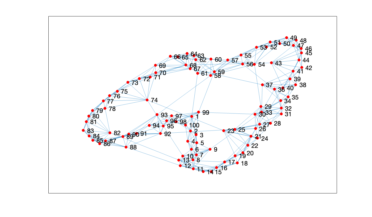
Because each node connects to relatively few others, the adjacency matrix is quite sparse.
spy(A)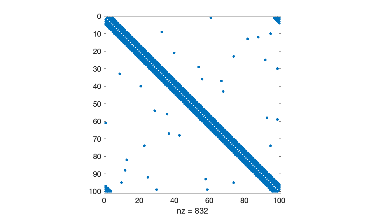
By Theorem 7.1.1, the entries of give the number of walks of length between pairs of nodes, as with “k degrees of separation” within a social network. As grows, the density of also grows.
clf
tiledlayout(2, 2)
for k = [2, 3, 4, 6]
    nexttile
    spy(A^k)
    title(sprintf("A^{%d}", k))
end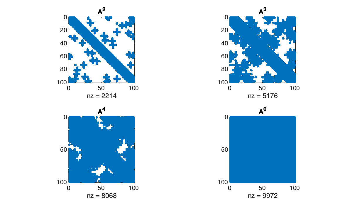
Example 8.1.2
Here is the adjacency matrix of a graph representing a small-world network, featuring connections to neighbors and a small number of distant contacts.
import networkx as nx
wsg = nx.watts_strogatz_graph(200, 4, 0.02)
Because each node connects to relatively few others, the adjacency matrix is quite sparse.
A = nx.adjacency_matrix(wsg)
spy(A)
title("Adjacency matrix $A$");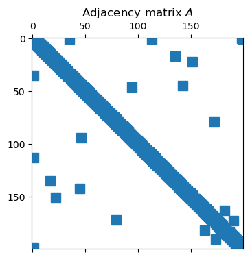
By Theorem 7.1.1, the entries of give the number of walks of length between pairs of nodes, as with “k degrees of separation” within a social network. As grows, the density of also grows.
Tip
While A**6 is valid syntax here, it means elementwise power, not matrix power.
from scipy.sparse.linalg import matrix_power
spy(matrix_power(A, 6))
title(("$A^6$"));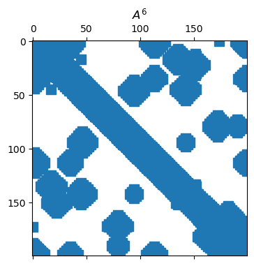
8.1.2Banded matrices
A particularly important type of sparse matrix is a banded matrix. Recall from Exploiting matrix structure that has upper bandwidth if implies , and lower bandwidth if implies . We say the total bandwidth is . Banded matrices appear naturally in many applications where each element interacts directly with only a few neighbors.
Without pivoting, an LU factorization preserves bandwidth, but pivoting can change or destroy bandedness.
Example 8.1.3
The spdiagm function creates a sparse matrix given its diagonal elements. The main or central diagonal is numbered zero, above and to the right of that is positive, and below and to the left is negative.
n = 50;
A = spdiagm(-3 => fill(n, n - 3),
    0 => ones(n),
    1 => -(1:n-1),
    5 => fill(0.1, n - 5))
Matrix(A[1:7, 1:7])
7×7 Matrix{Float64}:
1.0 -1.0 0.0 0.0 0.0 0.1 0.0
0.0 1.0 -2.0 0.0 0.0 0.0 0.1
0.0 0.0 1.0 -3.0 0.0 0.0 0.0
50.0 0.0 0.0 1.0 -4.0 0.0 0.0
0.0 50.0 0.0 0.0 1.0 -5.0 0.0
0.0 0.0 50.0 0.0 0.0 1.0 -6.0
0.0 0.0 0.0 50.0 0.0 0.0 1.0Without pivoting, the LU factors have the same lower and upper bandwidth as the original matrix.
Tip
The sparse function converts any matrix to sparse form. But it’s usually better to construct a sparse matrix directly, as the standard form might not fit in memory.
L, U = FNC.lufact(A)
plot(layout=2)
spy!(sparse(L), m=2, subplot=1, title=L"\mathbf{L}", color=:blues)
spy!(sparse(U), m=2, subplot=2, title=L"\mathbf{U}", color=:blues)However, if we introduce row pivoting, bandedness may be expanded or destroyed.
fact = lu(A)
plot(layout=2)
spy!(sparse(fact.L), m=2, subplot=1, title=L"\mathbf{L}", color=:blues)
spy!(sparse(fact.U), m=2, subplot=2, title=L"\mathbf{U}", color=:blues)Example 8.1.3
The spdiags function creates a sparse matrix given its diagonal elements. The main or central diagonal is numbered zero, above and to the right of that is positive, and below and to the left is negative.
n = 50;
n = 50;
% Put constant values on 3 diagonals
A = spdiags([n, 1, 0.1], [-3, 0, 5], n, n);
% Put other values on 1st superdiagonal
A = spdiags(-(0:n-1)', 1, A);
full(A(1:7, 1:7))Without pivoting, the LU factors have the same lower and upper bandwidth as the original matrix.
Tip
The sparse function converts any matrix to sparse form. But it’s usually better to construct a sparse matrix directly, as the standard form might not fit in memory.
[L, U] = lufact(A);
clf
subplot(1, 2, 1), spy(L), title('L')
subplot(1, 2, 2), spy(U), title(('U'));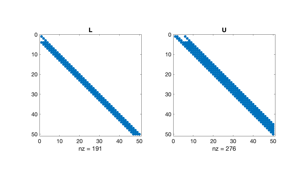
However, if we introduce row pivoting, bandedness may be expanded or destroyed.
[L, U, p] = plufact(A);
subplot(1, 2, 1), spy(L(p, :)), title('L')
subplot(1, 2, 2), spy(U), title(('U'));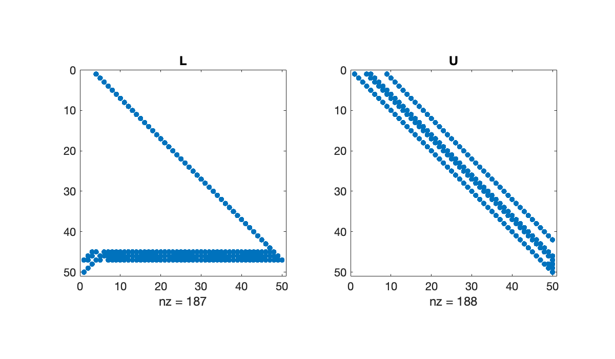
Example 8.1.3
The scipi.sparse.diags function creates a sparse matrix given its diagonal elements and the diagonal indexes to put them on. The main or central diagonal is numbered zero, above and to the right of that is positive, and below and to the left is negative.
n = 50
data = [n * ones(n-3), ones(n), linspace(-1, 1-n, n-1)]
offsets = [-3, 0, 1]    # 3rd below, main, 1st above
A = sp.diags(data, offsets, format="lil")
print(A[:7, :7].todense())
[[ 1. -1. 0. 0. 0. 0. 0.]
[ 0. 1. -2. 0. 0. 0. 0.]
[ 0. 0. 1. -3. 0. 0. 0.]
[50. 0. 0. 1. -4. 0. 0.]
[ 0. 50. 0. 0. 1. -5. 0.]
[ 0. 0. 50. 0. 0. 1. -6.]
[ 0. 0. 0. 50. 0. 0. 1.]]
Without pivoting, the LU factors have the same lower and upper bandwidth as the original matrix.
L, U = FNC.lufact(A.todense())
subplot(1, 2, 1), spy(L)
subplot(1, 2, 2), spy(U);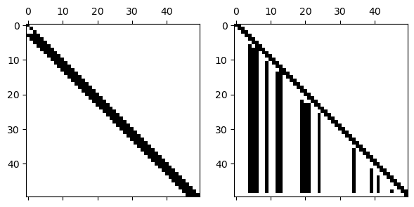
However, if we introduce row pivoting, bandedness may be expanded or destroyed.
L, U, p = FNC.plufact(A.todense())
subplot(1, 2, 1), spy(L[p, :])
subplot(1, 2, 2), spy(U)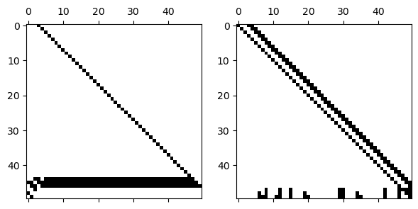
8.1.3Systems and eigenvalues
If given a sparse matrix, the backslash operator will automatically try a form of sparse-aware Cholesky or pivoted LU factorization. Depending on the sparsity pattern of the matrix, the time taken to solve the linear system may be well below the needed in the general case.
For very large matrices, it’s unlikely that you will want to find all of its eigenvalues and eigenvectors. In Krylov subspaces we describe some of the math behind an algorithm that can find a selected number of eigenvalues of largest magnitude, lying to the extreme left or right, or nearest a given complex number.
Example 8.1.4
The following generates a random sparse matrix with prescribed eigenvalues.
n = 4000
density = 4e-4
λ = @. 1 + 1 / (1:n)   # exact eigenvalues
A = FNC.sprandsym(n, density, λ);
The eigs function from Arpack finds a small number eigenvalues meeting some criterion. First, we ask for the 5 of largest (complex) magnitude using which=:LM.
using Arpack
λmax, V = eigs(A, nev=5, which=:LM)    # Largest Magnitude
formatters = [fmt__printf("%20.15f")]
column_labels=["found", "exact"]
pretty_table([λmax λ[1:5]];
column_labels, formatters, backend=:html)Now we find the 5 closest to the value 1 in the complex plane, via sigma=1.
λ1, V = eigs(A, nev=5, sigma=1)    # closest to sigma
data = [λ1 λ[end:-1:end-4]]
pretty_table(data; column_labels, formatters, backend=:html)The time needed to solve a sparse linear system is not easy to predict unless you have some more information about the matrix. But it will typically be orders of magnitude faster than the dense version of the same problem.
x = @. 1 / (1:n);
b = A * x;
norm(x - A \ b); # force compilation
t = @elapsed sparse_err = norm(x - A \ b)
println("Time for sparse solve: $t")Time for sparse solve: 0.00057425
D = Matrix(A)  # convert to regular matrix
norm(x - D \ b);
t = @elapsed dense_err = norm(x - D \ b)
println("Time for dense solve: $t")
Time for dense solve: 32.053302291
@show sparse_err;
@show dense_err;
sparse_err = 1.1782555574088238e-16
dense_err = 3.8074642587312435e-18
Example 8.1.4
The following generates a random sparse matrix with prescribed eigenvalues.
n = 4000;
density = 4e-4;
lambda = 1 ./ (1:n);
A = sprandsym(n, density, lambda);
clf,  spy(A)
title('Sparse symmetric matrix')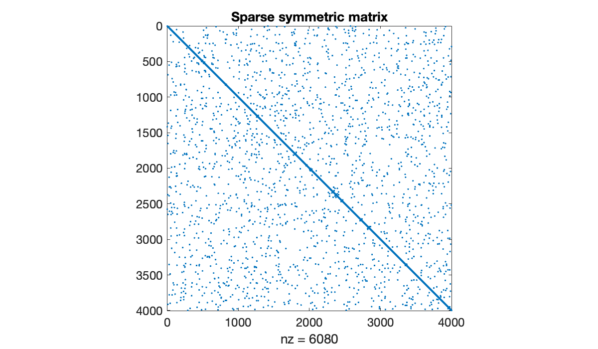
The eigs function finds a small number eigenvalues meeting some criterion. First, we ask for the 5 of largest (complex) magnitude.
[V, D] = eigs(A, 5);    % largest magnitude
1 ./ diag(D) % should be 1, 2, 3, 4, 5Now we find the 4 closest to the value 0.03 in the complex plane.
[V, D] = eigs(A, 4, 0.03);    % closest to 0.03
diag(D)The time needed to solve a sparse linear system is not easy to predict unless you have some more information about the matrix. But it will typically be orders of magnitude faster than the dense version of the same problem.
x = 1 ./ (1:n)';
b = A * x;
tic, sparse_err = norm(x - A\b), sparse_time = tocF = full(A);
tic, dense_err = norm(x - F\b), dense_time = tocExample 8.1.4
The following generates a random sparse matrix with prescribed eigenvalues.
n = 4000
density = 4e-4
ev = 1 / arange(1, n + 1)
A = FNC.sprandsym(n, density, eigvals=ev)
print(f"density is {A.nnz / prod(A.shape):.3%}")
density is 0.040%
The eigs function finds a small number eigenvalues meeting some criterion. First, we ask for the 5 of largest (complex) magnitude using which="LM".
from scipy.sparse.linalg import eigs
ev, V = eigs(A, k=5, which="LM")    # largest magnitude
print(1 / ev)
[1.+0.j 2.+0.j 3.+0.j 4.+0.j 5.+0.j]
Now we find the 4 closest to the value 1 in the complex plane, via sigma=1.
from scipy.sparse.linalg import eigs
ev, V = eigs(A, k=4, sigma=0.03)    # closest to sigma
print(ev)
[0.03030303+0.j 0.02941176+0.j 0.03125 +0.j 0.02857143+0.j]
The time needed to solve a sparse linear system is not easy to predict unless you have some more information about the matrix. But it will typically be orders of magnitude faster than the dense version of the same problem.
from scipy.sparse.linalg import spsolve
x = 1 / arange(1, n + 1)
b = A @ x
start = timer()
xx = spsolve(A, b)
print(f"sparse time: {timer() - start:.3g} sec")
print(f"residual: {norm(b - A @ xx, 2):.1e}")
sparse time: 0.000553 sec
residual: 7.7e-19
from scipy.linalg import solve
F = A.todense()
start = timer()
xx = solve(F, b)
print(f"dense time: {timer() - start:.3g} sec")
print(f"residual: {norm(b - A @ xx, 2):.1e}")
dense time: 0.249 sec
residual: 6.7e-19
8.1.4Exercises
⌨ Use spdiagm to build the matrices
For each matrix, use spy and an inspection of the submatrices in the corners to verify the correctness of your matrices.
⌨ This problem requires the matrix used in Example 8.1.2.
Download a data file by clicking the link.
using MAT
A = matread("smallworld.mat")["A"]
Download a data file by clicking the link.
load smallworldDownload a data file by right-clicking the link and selecting “Save As...”.
import scipy.io as spio
A = spio.mmread("smallworld.mtx")
(a) Find the density of (number of nonzeros divided by total number of elements), , , and . (You should find that it increases with the power of .)
(b) The LU factors tend to at least partially retain sparsity. Find the density of the and factors of using lufact (Algorithm 2.4.1). (If you get an error, convert the matrix to dense form first.)
(c) Repeat part (b) for the QR factorization using qrfact (Algorithm 3.4.1). (If you get an error, convert the matrix to dense form first.)
⌨ One use of adjacency matrices is to analyze the links between members of a collection. Obtain the adjacency matrix from Example 8.1.1 via the following:
Download roswell.mat by clicking the link and saving (you may need to fix the file name).
using MAT
A = matread("roswell.mat")["A"]
Download roswell.mat by clicking the link and saving (you may need to fix the file name).
load roswellDownload roswell.mtx by clicking the link and saving (you may need to fix the file name).
import scipy.io as spio
A = spio.mmread("roswell.mtx")
The matrix catalogs the links between web sites related to the town of Roswell, NM, with if and only if site links to site .
(a) Verify numerically that the matrix does not include any links from a site to itself.
(b) Verify numerically that is not symmetric. (Thus, its graph is a directed one.)
(c) How many sites in the group are not pointed to by any other sites in the group?
(d) Which site points to the most other sites?
(e) Which site is pointed to the most by the other sites? This is a crude way to establish the most important site.
(f) There are 27902 possible ways to connect ordered pairs of sites. What fraction of these pairs is connected by a walk of links that is no greater than three in length?
⌨ The graph Laplacian matrix is , where is the adjacency matrix and is the degree matrix, a diagonal matrix with diagonal entries .
Follow the directions in Exercise 8.1.3 to obtain an adjacency matrix . Then find the five eigenvalues of having largest magnitude.
⌨ See Exercise 7.1.5 for instructions on loading a matrix that contains information about the appearances of 392,400 actors in 127,823 movies, as given by the Internet Movie Database. Specifically, if actor appeared in movie , and all other elements are zero.
(a) What is the maximum number of actors appearing in any one movie?
(b) How many actors appeared in exactly three movies?
(c) Define . How many nonzero entries does have? What is the interpretation of ?
⌨ A matrix that arises from the Helmholtz equation for wave propagation can be specified using
A = FNC.poisson(n) - k^2*I;where is a real parameter. Let .
(a) Let . What is the size of ? What is its density?
(b) Still with , use eigs to find the four largest and four smallest (in magnitude) eigenvalues of . (See Example 8.1.4 for examples.)
(c) The eigenvalues are all real. Find a value of so that has exactly three negative eigenvalues.