from numpy import *
from scipy import linalg
from scipy.linalg import norm
from matplotlib.pyplot import *
from prettytable import PrettyTable
from timeit import default_timer as timer
import sys
sys.path.append('fncbook/')
import fncbook as FNC

# This (optional) block is for improving the display of plots.
# from IPython.display import set_matplotlib_formats
# set_matplotlib_formats("svg","pdf")
# %config InlineBackend.figure_format = 'svg'
rcParams["figure.figsize"] = [7, 4]
rcParams["lines.linewidth"] = 2
rcParams["lines.markersize"] = 4
rcParams['animation.html'] = "jshtml"  # or try "html5"

11.2.The method of lines¶

Our strategy in Black–Scholes equation was to discretize both the time and space derivatives using finite differences, then rearrange so that we could march the solution forward through time. It was partially effective, but as Example 11.1.3 shows, not a sure thing, for reasons we look into starting in the next section.

First, though, we want to look at a broader version of the discretization approach. To introduce ideas, let’s use the simpler heat equation, $u_t = u_{xx}$ , as a model. Because boundaries always complicate things, we will start by doing the next best thing to having no boundaries at all: periodic end conditions. Specifically, we will solve the PDE over $0\le x < 1$ and require at all times that

u(x+1,t)=u(x,t) \quad \text{for all $x$}.

(11.2.1)

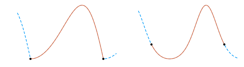
This is a little different from simply $u(1,t)=u(0,t)$ , as Figure 11.2.1 illustrates.

periodic function illustration — Figure 11.2.1:Left: A function whose values are the same at the endpoints of an interval does not necessarily extend to a smooth periodic function. Right: For a truly periodic function, the function values and all derivatives match at the endpoints of one period.

11.2.1Semidiscretization¶

As a reminder, we use $\hat{u}$ when we specifically refer to the exact solution of the PDE. In order to avoid carrying along redundant information about the function, we use $x_i = ih$ only for $i=0,\ldots,m-1$ , where $h=1/m$ , and it’s understood that a reference to $x_m$ is silently translated to one at $x_0$ . More generally, we have the identity

\hat{u}(x_i,t) = \hat{u}\bigl(x_{(i \bmod{m})},t \bigr)

(11.2.2)

for the exact solution $\hat{u}$ at any value of $i$ .

Next we define a vector $\mathbf{u}$ by

\mathbf{u}(t) = \begin{bmatrix} u_0(t) \\ u_1(t) \\ \vdots \\ u_{m-1}(t) \end{bmatrix}.

(11.2.3)

This step is called semidiscretization, since space is discretized but time is not. As in Chapter 10, we will replace $u_{xx}$ with multiplication of $\mathbf{u}$ by a differentiation matrix $\mathbf{D}_{xx}$ . The canonical choice is the three-point finite-difference formula (5.4.9), which in light of the periodicity (11.2.2) leads to

\mathbf{D}_{xx} = \frac{1}{h^2} \begin{bmatrix} -2 & 1 & & & 1 \\ 1 & -2 & 1 & & \\ & \ddots & \ddots & \ddots & \\ & & 1 & -2 & 1 \\ 1 & & & 1 & -2 \end{bmatrix}.

(11.2.4)

Note well how the first and last rows have elements that “wrap around” from one end of the domain to the other by periodicity. Because we will be using this matrix quite a lot, we create Function 11.2.1 to compute it, as well as the corresponding second-order first derivative matrix $\mathbf{D}_x$ for periodic end conditions.

Algorithm 11.2.1 (diffper)

diffper.py

1
2
3
4
5
6
7
8
9
10
11
12
13
14
15
16
17
18
19
20
21
22
23
24
25
26
27
def diffper(n, xspan):
    """
    diffper(n, xspan)

    Construct 2nd-order differentiation matrices for functions with periodic end
    conditions, using `n` unique nodes in the interval `xspan`. Return a vector of
    nodes and the  matrices for the first and second derivatives.
    """
    a, b = xspan
    h = (b - a) / n
    x = a + h * np.arange(n)  # nodes, omitting the repeated data

    # Construct Dx by diagonals, then correct the corners.
    dp = 0.5 / h * np.ones(n - 1)  # superdiagonal
    dm = -0.5 / h * np.ones(n - 1)  # subdiagonal
    Dx = np.diag(dm, -1) + np.diag(dp, 1)
    Dx[0, -1] = -1 / (2 * h)
    Dx[-1, 0] = 1 / (2 * h)

    # Construct Dxx by diagonals, then correct the corners.
    d0 = -2 / h**2 * np.ones(n)  # main diagonal
    dp = np.ones(n - 1) / h**2  # superdiagonal and subdiagonal
    Dxx = np.diag(d0) + np.diag(dp, -1) + np.diag(dp, 1)
    Dxx[0, -1] = 1 / (h**2)
    Dxx[-1, 0] = 1 / (h**2)

    return x, Dx, Dxx

The PDE $u_t=u_{xx}$ is now approximated by the semidiscrete problem

\frac{d \mathbf{u}(t)}{d t} = \mathbf{D}_{xx} \mathbf{u}(t),

(11.2.5)

which is simply a linear, constant-coefficient system of ordinary differential equations. Given the initial values $\mathbf{u}(0)$ obtained from $u(x_i,0)$ , we have an initial-value problem that we already know how to solve!

Semidiscretization is often called the method of lines. Despite the name, it is not exactly a single method because both space and time discretizations have to be specified in order to get a concrete algorithm. The key concept is the separation of those two discretizations, and in that way, it’s related to separation of variables in analytic methods for the heat equation.

Example 11.2.1

Suppose we solve (11.2.5) using the Euler IVP integrator (6.2.5) from Euler’s method (and also AB1 from Multistep methods). We select a time step $\tau$ and discrete times $t_j=j\tau$ , $j=0,1,\ldots,n$ . We can discretize the vector $\mathbf{u}$ in time as well to get a sequence $\mathbf{u}_j \approx \mathbf{u}(t_j)$ for varying $j$ . (Remember the distinction in notation between $\mathbf{u}_j$ , which is a vector, and $u_j$ , which is a single element of a vector.)

Thus, a fully discrete method for the heat equation is

\mathbf{u}_{j+1} = \mathbf{u}_j + \tau ( \mathbf{D}_{xx} \mathbf{u}_j) = (\mathbf{I} + \tau \mathbf{D}_{xx} ) \mathbf{u}_j.

(11.2.6)

Example 11.2.2 (Forward Euler for the heat equation)

Let’s implement the method of Example 11.2.1 with second-order space semidiscretization.

m = 100
x, Dx, Dxx = FNC.diffper(m, [0, 1])

tfinal = 0.15  
n = 2400                 # number of time steps  
tau = tfinal / n         # time step
t = tau * arange(n+1)    # time values

Next we set an initial condition. It isn’t mathematically periodic, but the end values and derivatives are so small that for numerical purposes it may as well be.

U = zeros([m, n+1])
U[:, 0] = exp(-60 * (x - 0.5) ** 2)
plot(x, U[:, 0])
xlabel("x");  ylabel("u(x,0)")
title("Initial condition");

The Euler time stepping simply multiplies the solution vector by the constant matrix in (11.2.6) at each time step. Since that matrix is sparse, we will declare it as such, even though the run-time savings may not be detectable for this small value of $m$ .

import scipy.sparse as sp
I = sp.eye(m)
A = I + tau * sp.csr_array(Dxx)
for j in range(n):
    U[:, j+1] = A @ U[:, j]

plot(x, U[:, :31:10])
ylim([-0.25, 1])
xlabel("$x$");  ylabel("$u(x,t)$")
legend([f"$t={tj:.2e}$" for tj in t[:60:20]])
title("Heat equation by forward Euler");

You see above that things seem to start well, with the initial peak widening and shrinking. But then there is a nonphysical growth in the solution.

from matplotlib import animation
fig = figure()
ax = fig.add_subplot(autoscale_on=False, xlim=(0, 1), ylim=(-1, 2))
ax.grid()

line, = ax.plot([], [], '-', lw=2)
ax.set_title("Heat equation by forward Euler")
time_text = ax.text(0.05, 0.9, '', transform=ax.transAxes)

def animate(j):
    line.set_data(x, U[:, j])
    time_text.set_text(f"t = {t[j]:.2e}")
    return line, time_text

anim = animation.FuncAnimation(
    fig, animate, frames=range(0, 100), blit=True)
anim.save("diffusionFE.mp4", fps=24)
close()

The growth in norm is exponential in time.

M = abs(U).max(axis=0)  # max in each column
semilogy(t[:500], M[:500])
xlabel("$t$");  ylabel("$\\max_x |u(x,t)|$")
title("Nonphysical growth");

The method in Example 11.2.1 and Example 11.2.2 is essentially the same one we used for the Black–Scholes equation in Black–Scholes equation. By changing the time integrator, we can get much better results.

Example 11.2.4 (Backward Euler for the heat equation)

Now we apply backward Euler to the heat equation. Mathematically this means multiplying by the inverse of a matrix, but we interpret that numerically as a linear system solution. We will reuse the setup from Example 11.2.2.

from scipy.sparse.linalg import spsolve
B = sp.csr_matrix(I - tau * Dxx)
for j in range(n):
    U[:, j + 1] = spsolve(B, U[:, j])

plot(x, U[:, ::500])
xlabel("$x$")
ylabel("$u(x,t)$")
legend([f"$t={tj:.2g}$" for tj in t[::500]])
title("Heat equation by backward Euler");

fig = figure()
ax = fig.add_subplot(autoscale_on=False, xlim=(0, 1), ylim=(-0.25, 1))
ax.grid()

line, = ax.plot([], [], '-', lw=2)
ax.set_title("Backward Euler")
time_text = ax.text(0.05, 0.9, '', transform=ax.transAxes)

anim = animation.FuncAnimation(
    fig, animate, frames=range(0, n+1, 20), blit=True)
anim.save("diffusionBE.mp4", fps=30)
close()

This solution looks physically plausible, as the large concentration in the center diffuses outward until the solution is essentially constant. Observe that the solution remains periodic in space for all time.

Example 11.2.4 suggests that implicit time stepping methods have an important role in diffusion. We will analyze the reason in the next few sections.

11.2.2Black-box IVP solvers¶

Instead of coding one of the Runge–Kutta or multistep formulas directly for a method of lines solution, we could use any of the IVP solvers from Chapter 6, or a solver from the DifferentialEquations package, to solve the ODE initial-value problem (11.2.5).

Example 11.2.5 (Adaptive time stepping for the heat equation)

We set up the semidiscretization and initial condition in $x$ just as before.

m = 100
x, Dx, Dxx = FNC.diffper(m, [0, 1])
u0 = exp(-60 * (x - 0.5) ** 2)

Now, however, we apply a standard solver using solve_ivp to the initial-value problem $\mathbf{u}'=\mathbf{D}_{xx}\mathbf{u}$ .

from scipy.integrate import solve_ivp
tfinal = 0.05
f = lambda t, u: Dxx @ u
sol = solve_ivp(f, [0, tfinal], u0, method="RK45", dense_output=True)

t = linspace(0, 0.05, 5)
plot(x, sol.sol(t))
xlabel("$x$"),  ylabel("$u(x,t)$")
legend([f"$t={tj:.4g}$" for tj in t])
title("Heat equation by RK45");

The solution appears to be correct. But the number of time steps that were selected automatically is surprisingly large, considering how smoothly the solution changes.

print(f"RK45 took {len(sol.t) - 1} steps")

RK45 took 602 steps

Now we apply a different solver called BDF.

sol = solve_ivp(f, [0, tfinal], u0, method="BDF")
print(f"BDF took {len(sol.t) - 1} steps")

BDF took 34 steps

The number of steps selected was reduced by a factor of 20!

The adaptive time integrators can all produce solutions. But, as seen in Example 11.2.5, they are not equivalent in every important sense. Whether we choose to implement a method directly with a fixed step size, or automatically with adaptation, there is something crucial to understand about the semidiscrete problem (11.2.5) that will occupy our attention in the next two sections.

11.2.3Exercises¶

Exercise 11.2.6

✍ In this problem, you will analyze the convergence of the explicit method given by (11.2.6). Recall that the discrete approximation $u_{i,j}$ approximates the solution at $x_i$ and $t_j$ .

(a) Write the method in scalar form as

u_{i,j+1} = (1-2\lambda) u_{i,j} + \lambda u_{i+1,j} + \lambda u_{i-1,j},

(11.2.9)

where $\lambda = \tau/h^2>0$ .

(b) Taylor series of the exact solution $\hat{u}$ imply that

\begin{align*} \hat{u}_{i,j+1} &= \hat{u}_{i,j} + \frac{\partial \hat{u}}{\partial t} (x_i,t_j) \tau + O(\tau^2),\\ % \frac{\partial^2 u}{\partial t^2} (x_i,\bar{t}) \frac{\tau^2}{2} \hat{u}_{i\pm1,j} &= \hat{u}_{i,j} \pm \frac{\partial \hat{u}}{\partial x} (x_i,t_j) h + \frac{\partial^2 \hat{u}}{\partial x^2} (x_i,t_j) \frac{h^2}{2} \pm \frac{\partial^3 \hat{u}}{\partial x^3} (x_i,t_j) \frac{h^3}{6}+ O(h^4). %\frac{\partial^4 u}{\partial x^4} (\bar{x}_\pm,t_j) \frac{h^4}{24}. \end{align*}

(11.2.10)

Use these to show that

\begin{align*} \hat{u}_{i,j+1} & = \left[ (1-2\lambda) \hat{u}_{i,j} + \lambda \hat{u}_{i+1,j} + \lambda \hat{u}_{i-1,j}\right] + O\Bigl(\tau^2+h^2 \Bigr)\\ &= F\left( \lambda,\hat{u}_{i,j}, \hat{u}_{i+1,j} , \hat{u}_{i-1,j}\right) + O\Bigl(\tau^2+h^2\Bigr). \end{align*}

(11.2.11)

(The last line should be considered a definition of the function $F$ .)

(c) The numerical solution satisfies

u_{i,j+1}=F\bigl( \lambda,u_{i,j}, u_{i+1,j} , u_{i-1,j}\bigr)

(11.2.12)

exactly. Using this fact, subtract $u_{i,j+1}$ from both sides of the last line in part (b) to show that

e_{i,j+1} = F\left( \lambda,e_{i,j}, e_{i+1,j} ,e_{i-1,j}\right) + O\Bigl(\tau^2+h^2\Bigr),

(11.2.13)

where $e_{i,j}=\hat{u}_{i,j}-u_{i,j}$ is the error in the numerical solution for all $i$ and $j$ .

(d) Define $E_j$ as the maximum of $|e_{i,j}|$ over all values of $i$ , and use the result of part (c) to show that if $\lambda<1/2$ is kept fixed as $h$ and $\tau$ approach zero, then for sufficiently small $\tau$ and $h$ ,

E_{j+1} = E_{j} + O\Bigl(\tau^2+h^2\Bigr) \le E_{j} + K_j\bigl(\tau^2+h^2\bigr)

(11.2.14)

for a positive $K_j$ independent of $\tau$ and $h$ .

(e) If the initial conditions are exact, then $E_0=0$ . Use this to show finally that if the $K_j$ are bounded above and $\lambda<1/2$ is kept fixed, then $E_n = O(\tau)$ as $\tau\to 0$ .