from numpy import *
from scipy import linalg
from scipy.linalg import norm
from matplotlib.pyplot import *
from prettytable import PrettyTable
from timeit import default_timer as timer
import sys
sys.path.append('fncbook/')
import fncbook as FNC

# This (optional) block is for improving the display of plots.
# from IPython.display import set_matplotlib_formats
# set_matplotlib_formats("svg","pdf")
# %config InlineBackend.figure_format = 'svg'
rcParams["figure.figsize"] = [7, 4]
rcParams["lines.linewidth"] = 2
rcParams["lines.markersize"] = 4
rcParams['animation.html'] = "jshtml"  # or try "html5"

5.6.Numerical integration¶

In calculus, you learn that the elegant way to evaluate a definite integral is to apply the Fundamental Theorem of Calculus and find an antiderivative. The connection is so profound and pervasive that it’s easy to overlook that a definite integral is a numerical quantity existing independently of antidifferentiation. However, most conceivable integrands have no antiderivative in terms of familiar functions.

Example 5.6.1 (Numerical integration)

The antiderivative of $e^x$ is, of course, itself. That makes evaluation of $\int_0^1 e^x\,dx$ by the Fundamental Theorem trivial.

exact = exp(1) - 1

The module scipy.integrate has multiple functions that estimate the value of an integral numerically without finding the antiderivative first. As you can see here, it’s often just as accurate.

from scipy.integrate import quad
Q, errest = quad(exp, 0, 1, epsabs=1e-13, epsrel=1e-13)
print(Q)

1.7182818284590453

The numerical approach is also far more robust. For example, $e^{\,\sin x}$ has no useful antiderivative. But numerically, it’s no more difficult.

Q, errest = quad(lambda x: exp(sin(x)), 0, 1, epsabs=1e-13, epsrel=1e-13)
print(Q)

1.6318696084180513

When you look at the graphs of these functions, what’s remarkable is that one of these areas is basic calculus while the other is almost impenetrable analytically. From a numerical standpoint, they are practically the same problem.

x = linspace(0, 1, 300)
subplot(1, 2, 1)
plot(x, exp(x))
ylim([0, 2.7]), title("exp(x)")
subplot(1, 2, 2)
plot(x, exp(sin(x)))
ylim([0, 2.7]), title("exp(sin(x))");

Numerical integration, which also goes by the older name quadrature, is performed by combining values of the integrand sampled at nodes. In this section we will assume equally spaced nodes using the definitions

t_i = a +i h, \quad h=\frac{b-a}{n}, \qquad i=0,\ldots,n.

(5.6.1)

Numerical integration formulas can be applied to sequences of data values even if no function is explicitly known to generate them. For our presentation and implementations, however, we assume that $f$ is known and can be evaluated anywhere.

A straightforward way to derive integration formulas is to mimic the approach taken for finite differences: find an interpolant and operate exactly on it.

5.6.1Trapezoid formula¶

One of the most important integration formulas results from integration of the piecewise linear interpolant (see Piecewise linear interpolation). Using the cardinal basis form of the interpolant in (5.2.3), we have

\int_a^b f(x) \, dx \approx \int_a^b \sum_{i=0}^n f(t_i) H_i(x)\, dx = \sum_{i=0}^n f(t_i) \left[ \int_a^b H_i(x)\, dx \right].

(5.6.3)

Thus, we can identify the weights as $w_i = h^{-1} \int_a^b H_i(x)\, dx$ . Using areas of triangles, it’s trivial to derive that

w_i = \begin{cases} 1, & i=1,\ldots,n-1,\\ \frac{1}{2}, & i=0,n. \end{cases}

(5.6.4)

Putting everything together, the resulting formula is

\begin{split} \int_a^b f(x)\, dx \approx T_f(n) &= h\left[ \frac{1}{2}f(t_0) + f(t_1) + f(t_2) + \cdots + f(t_{n-1}) + \frac{1}{2}f(t_n) \right]. \end{split}

(5.6.5)

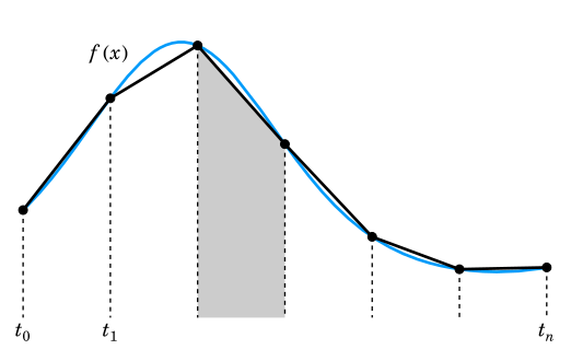
Geometrically, as illustrated in Figure 5.6.1, the trapezoid formula sums of the areas of trapezoids approximating the region under the curve $y=f(x)$ .^[1]

The trapezoid formula is the Swiss Army knife of integration formulas. A short implementation is given as Function 5.6.1.

Figure 5.6.1:Trapezoid formula for integration. The piecewise linear interpolant defines trapezoids that approximate the region under the curve.

Algorithm 5.6.1 (trapezoid)

trapezoid.py

1
2
3
4
5
6
7
8
9
10
11
def trapezoid(f, a, b, n):
    """
    trapezoid(f, a, b, n)

    Apply the trapezoid integration formula for integrand f over interval [a,b], broken up into n equal pieces. Returns estimate, vector of nodes, and vector of integrand values at the nodes.
    """
    h = (b - a) / n
    t = np.linspace(a, b, n + 1)
    y = f(t)
    T = h * (np.sum(y[1:-1]) + 0.5 * (y[0] + y[-1]))
    return T, t, y

Like finite-difference formulas, numerical integration formulas have a truncation error.

In Theorem 5.2.2 we stated that the pointwise error in a piecewise linear interpolant with equal node spacing $h$ is bounded by $O(h^2)$ as $h\rightarrow 0$ . Using $I$ to stand for the exact integral of $f$ and $p$ to stand for the piecewise linear interpolant, we obtain

\begin{split} I - T_f(n) = I - \int_a^b p(x)\, dx &= \int_a^b \bigl[f(x)-p(x)\bigr] \, dx \\ &\le (b-a) \max_{x\in[a,b]} |f(x)-p(x)| = O(h^2). \end{split}

(5.6.8)

A more thorough statement of the truncation error is known as the Euler–Maclaurin formula,

\begin{split} \int_a^b f(x)\, dx &= T_f(n) - \frac{h^2}{12} \left[ f'(b)-f'(a) \right] + \frac{h^4}{720} \left[ f'''(b)-f'''(a) \right] + O(h^6) \\ &= T_f(n) - \sum_{k=1}^\infty \frac{B_{2k}h^{2k}}{(2k)!} \left[ f^{(2k-1)}(b)-f^{(2k-1)}(a) \right], \end{split}

(5.6.9)

where the $B_{2k}$ are constants known as Bernoulli numbers. Unless we happen to be fortunate enough to have a function with $f'(b)=f'(a)$ , we should expect truncation error at second order and no better.

Example 5.6.2 (Trapezoid integration)

We will approximate the integral of the function $f(x)=e^{\sin 7x}$ over the interval $[0,2]$ .

f = lambda x: exp(sin(7 * x))
a, b = 0, 2

In lieu of the exact value, we will use the quad function to find an accurate result.

from scipy.integrate import quad
I, errest = quad(f, a, b, epsabs=1e-13, epsrel=1e-13)
print(f"Integral = {I:.14f}")

Integral = 2.66321978276154

Here is the trapezoid result at $n=40$ , and its error.

T, t, y = FNC.trapezoid(f, a, b, 40)
print(f"Trapezoid estimate is {T:.14f} with error {I - T:.2e}")

Trapezoid estimate is 2.66230293560229 with error 9.17e-04

In order to check the order of accuracy, we increase $n$ by orders of magnitude and observe how the error decreases.

n_ = 40 * 2 ** arange(6)
err = zeros(size(n_))
print("     n     error")
for k, n in enumerate(n_):
    T, t, y = FNC.trapezoid(f, a, b, n)
    err[k] = I - T
    print(f"{n:6d}   {err[k]:8.3e} ")

     n     error
    40   9.168e-04 
    80   2.301e-04 
   160   5.757e-05 
   320   1.440e-05 
   640   3.599e-06 
  1280   8.998e-07

Each increase by a factor of 10 in $n$ cuts the error by a factor of about 100, which is consistent with second-order convergence. Another check is that a log-log graph should give a line of slope -2 as $n\to\infty$ .

loglog(n_, abs(err), "-o", label="results")
loglog(n_, 3e-3 * (n_ / n_[0]) ** (-2), "--", label="2nd order")
gca().invert_xaxis()
xlabel("$n$")
ylabel("error")
legend()
title("Convergence of trapezoidal integration");

5.6.2Extrapolation¶

If evaluations of $f$ are computationally expensive, we want to get as much accuracy as possible from them by using a higher-order formula. There are many routes for doing so; for example, we could integrate a not-a-knot cubic spline interpolant. However, splines are difficult to compute by hand, and as a result different methods were developed before computers came on the scene.

Knowing the structure of the error allows the use of extrapolation to improve accuracy. Suppose a quantity $A_0$ is approximated by an algorithm $A(h)$ with an error expansion

A_0 = A(h) + c_1 h + c_2 h^2 + c_3 h^3 + \cdots.

(5.6.10)

Crucially, it is not necessary to know the values of the error constants $c_k$ , merely that they exist and are independent of $h$ .

Using $I$ for the exact integral of $f$ , the trapezoid formula has

I = T_f(n) + c_2 h^2 + c_4 h^{4} + \cdots,

(5.6.11)

as proved by the Euler–Maclaurin formula (5.6.9). The error constants depend on $f$ and can’t be evaluated in general, but we know that this expansion holds. For convenience, we recast the error expansion in terms of $n=O(h^{-1})$ :

I = T_f(n) + c_2 n^{-2} + c_4 n^{-4} + \cdots.

(5.6.12)

We now make the simple observation that

I = T_f(2n) + \tfrac{1}{4} c_2 n^{-2} + \tfrac{1}{16} c_4 n^{-4} + \cdots.

(5.6.13)

It follows that if we combine (5.6.12) and (5.6.13) correctly, we can cancel out the second-order term in the error. Specifically, define

S_f(2n) = \frac{1}{3} \Bigl[ 4 T_f(2n) - T_f(n) \Bigr].

(5.6.14)

(We associate $2n$ rather than $n$ with the extrapolated result because of the total number of nodes needed.) Then

I - S_f(2n) = O(n^{-4}) = b_4 n^{-4} + b_6 n^{-6} + \cdots.

(5.6.15)

The formula (5.6.14) is called Simpson’s formula, or Simpson’s rule. A different presentation and derivation are considered in Exercise 5.6.4.

Equation (5.6.15) is another particular error expansion in the form (5.6.10), so we can extrapolate again! The details change only a little. Considering that

I - S_f(4n) = \tfrac{1}{16} b_4 n^{-4} + \tfrac{1}{64} b_6 n^{-6} + \cdots,

(5.6.16)

the proper combination this time is

R_f(4n) = \frac{1}{15} \Bigl[ 16 S_f(4n) - S_f(2n) \Bigr],

(5.6.17)

which is sixth-order accurate. Clearly the process can be repeated to get eighth-order accuracy and beyond. Doing so goes by the name of Romberg integration, which we will not present in full generality.

5.6.3Node doubling¶

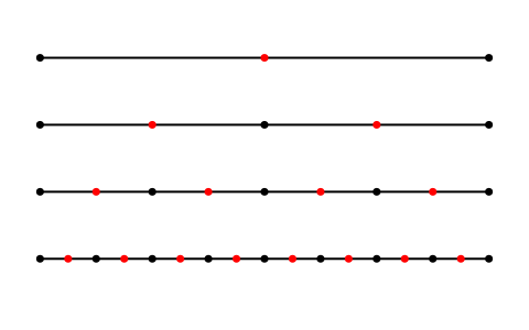
Note in (5.6.17) that $R_f(4n)$ depends on $S_f(2n)$ and $S_f(4n)$ , which in turn depend on $T_f(n)$ , $T_f(2n)$ , and $T_f(4n)$ . There is a useful benefit realized by doubling of the nodes in each application of the trapezoid formula. As shown in Figure 5.6.2, when doubling $n$ , only about half of the nodes are new ones, and previously computed function values at the other nodes can be reused.

Figure 5.6.2:Dividing the node spacing by half introduces new nodes only at midpoints, allowing the function values at existing nodes to be reused for extrapolation.

Specifically, we have

\begin{split} T_f(2m) & = \frac{1}{2m} \left[ \frac{1}{2} f(a) + \frac{1}{2} f(b) + \sum_{i=1}^{2m-1} f\Bigl( a + \frac{i}{2m} \Bigr) \right]\\[1mm] & = \frac{1}{2m} \left[ \frac{1}{2} f(a) + \frac{1}{2} f(b)\right] + \frac{1}{2m} \sum_{k=1}^{m-1} f\Bigl( a+\frac{2k}{2m} \Bigr) + \frac{1}{2m} \sum_{k=1}^{m} f\Bigl( a+\frac{2k-1}{2m} \Bigr) \\[1mm] &= \frac{1}{2m} \left[ \frac{1}{2} f(a) + \frac{1}{2} f(b) + \sum_{k=1}^{m-1} f\Bigl( a+\frac{k}{m} \Bigr) \right] + \frac{1}{2m} \sum_{k=1}^{m} f\Bigl( a+\frac{2k-1}{2m} \Bigr) \\[1mm] &= \frac{1}{2} T_f(m) + \frac{1}{2m} \sum_{k=1}^m f\left(t_{2k-1} \right), \end{split}

(5.6.18)

where the nodes referenced in the last line are relative to $n=2m$ . Hence in passing from $n=m$ to $n=2m$ , new integrand evaluations are needed only at the odd-numbered nodes of the finer grid.

Example 5.6.3 (Integration by extrapolation)

We estimate $\displaystyle\int_0^2 x^2 e^{-2x}\, dx$ using extrapolation. First we use quadgk to get an accurate value.

from scipy.integrate import quad
f = lambda x: x**2 * exp(-2 * x)
a = 0
b = 2
I, errest = quad(f, a, b, epsabs=1e-13, epsrel=1e-13)
print(f"Integral = {I:.14f}")

Integral = 0.19047417361161

We start with the trapezoid formula on $n=N$ nodes.

N = 20    # the coarsest formula
n = N
h = (b - a) / n
t = h * arange(n + 1)
y = f(t)

We can now apply weights to get the estimate $T_f(N)$ .

T = zeros(3)
T[0] = h * (sum(y[1:-1]) + y[0] / 2 + y[-1] / 2)
print(f"error (2nd order): {I - T[0]:.2e}")

error (2nd order): 6.27e-05

Now we double to $n=2N$ , but we only need to evaluate $f$ at every other interior node and apply (5.6.18).

n = 2 * n
h = h / 2
t = h * arange(n + 1)
T[1] = T[0] / 2 + h * sum(f(t[1:-1:2]))
print("error (2nd order):", I - T[:2])

error (2nd order): [6.27236723e-05 1.53677521e-05]

As expected for a second-order estimate, the error went down by a factor of about 4. We can repeat the same code to double $n$ again.

n = 2 * n
h = h / 2
t = h * arange(n + 1)
T[2] = T[1] / 2 + h * sum(f(t[1:-1:2]))
print("error (2nd order):", I - T[:3])

error (2nd order): [6.27236723e-05 1.53677521e-05 3.82230697e-06]

Let us now do the first level of extrapolation to get results from Simpson’s formula. We combine the elements T[i] and T[i+1] the same way for $i=1$ and $i=2$ .

S = array([(4 * T[i + 1] - T[i]) / 3 for i in range(2)])
print("error (4th order):", I - S)

error (4th order): [-4.17554646e-07 -2.61747412e-08]

With the two Simpson values $S_f(N)$ and $S_f(2N)$ in hand, we can do one more level of extrapolation to get a sixth-order accurate result.

R = (16 * S[1] - S[0]) / 15
print("error (6th order):", I - R)

error (6th order): -8.274758656057202e-11

We can make a triangular table of the errors:

results = PrettyTable()
results.add_column("2nd order", I - T)
results.add_column("4th order", concatenate(([nan],I - S)))
results.add_column("6th order", [nan, nan, I - R])
print(results)

+------------------------+-------------------------+------------------------+
|       2nd order        |        4th order        |       6th order        |
+------------------------+-------------------------+------------------------+
| 6.272367234608223e-05  |           nan           |          nan           |
| 1.5367752102174448e-05 | -4.1755464580406354e-07 |          nan           |
| 3.822306969658573e-06  | -2.6174741207807273e-08 | -8.274758656057202e-11 |
+------------------------+-------------------------+------------------------+

If we consider the computational time to be dominated by evaluations of $f$ , then we have obtained a result with about twice as many accurate digits as the best trapezoid result, at virtually no extra cost.

5.6.4Exercises¶

Exercise 5.6.1

⌨ For each integral below, use Function 5.6.1 to estimate the integral for $n=10\cdot 2^k$ nodes for $k=1,2,\ldots,10$ . Make a log-log plot of the errors and confirm or refute second-order accuracy. (These integrals were taken from Bailey et al. (2005).)

(a) $\displaystyle \int_0^1 x\log(1+x)\, dx = \frac{1}{4}$

(b) $\displaystyle \int_0^1 x^2 \tan^{-1}x\, dx = \frac{\pi-2+2\log 2}{12}$

(c) $\displaystyle \int_0^{\pi/2}e^x \cos x\, dx = \frac{e^{\pi/2}-1}{2}$

(d) $\displaystyle \int_0^1 \sqrt{x} \log(x) \, dx = -\frac{4}{9}$ (Note: Although the integrand has the limiting value zero as $x\to 0$ , it cannot be evaluated naively at $x=0$ . You can start the integral at $x=\macheps$ instead.)

(e) $\displaystyle \int_0^1 \sqrt{1-x^2}\,\, dx = \frac{\pi}{4}$

Exercise 5.6.2

✍ The Euler–Maclaurin error expansion (5.6.9) for the trapezoid formula implies that if we could cancel out the term due to $f'(b)-f'(a)$ , we would obtain fourth-order accuracy. We should not assume that $f'$ is available, but approximating it with finite differences can achieve the same goal. Suppose the 3-point forward difference formula in the second row of Table 5.4.2 is used for $f'(a)$ , and its reflected backward difference is used for $f'(b)$ . Show that the resulting modified trapezoid formula is

G_f(h) = T_f(h) - \frac{h}{24} \left[ 3\Bigl( f(t_n)+f(t_0) \Bigr) -4\Bigr( f(t_{n-1}) + f(t_1) \Bigr) + \Bigl( f(t_{n-2})+f(t_2) \Bigr) \right],

(5.6.19)

which is known as a Gregory integration formula.

Exercise 5.6.4

✍ Simpson’s formula can be derived without appealing to extrapolation.

(a) Show that

p(x) = \beta + \frac{\gamma-\alpha}{2h}\, x + \frac{\alpha-2\beta+\gamma}{2h^2}\, x^2

interpolates the three points $(-h,\alpha)$ , $(0,\beta)$ , and $(h,\gamma)$ .

(b) Find

\int_{-h}^h p(s)\, ds,

where $p$ is the quadratic polynomial from part (a), in terms of $h$ , $\alpha$ , $\beta$ , and $\gamma$ .

(c) Assume equally spaced nodes in the form $t_i=a+ih$ , for $h=(b-a)/n$ and $i=0,\ldots,n$ . Suppose $f$ is approximated by $p(x)$ over the subinterval $[t_{i-1},t_{i+1}]$ . Apply the result from part (b) to find

\int_{t_{i-1}}^{t_{i+1}} f(x)\, dx \approx \frac{h}{3} \bigl[ f(t_{i-1}) + 4f(t_i) + f(t_{i+1}) \bigr].

(5.6.20)

(Use the change of variable $s=x-t_i$ .)

(d) Now also assume that $n=2m$ for an integer $m$ . Derive Simpson’s formula,

\begin{split} \int_a^b f(x)\, dx \approx \frac{h}{3}\bigl[ &f(t_0) + 4f(t_1) + 2f(t_2) + 4f(t_3) + 2f(t_4) + \cdots\\ &+ 2f(t_{n-2}) + 4f(t_{n-1}) + f(t_n) \bigr]. \end{split}

(5.6.21)

Footnotes¶

Some texts distinguish between a formula for a single subinterval $[t_{k-1},t_k]$ and a composite formula that adds them up over the whole interval to get (5.6.5).
↩

References¶

Bailey, D. H., Jeyabalan, K., & Li, X. S. (2005). A Comparison of Three High-Precision Quadrature Schemes. Experimental Mathematics, 14(3), 317–329. 10.1080/10586458.2005.10128931