from numpy import *
from scipy import linalg
from scipy.linalg import norm
from matplotlib.pyplot import *
from prettytable import PrettyTable
from timeit import default_timer as timer
import sys
sys.path.append('fncbook/')
import fncbook as FNC

# This (optional) block is for improving the display of plots.
# from IPython.display import set_matplotlib_formats
# set_matplotlib_formats("svg","pdf")
# %config InlineBackend.figure_format = 'svg'
rcParams["figure.figsize"] = [7, 4]
rcParams["lines.linewidth"] = 2
rcParams["lines.markersize"] = 4
rcParams['animation.html'] = "jshtml"  # or try "html5"

3.3.The QR factorization¶

Sets of vectors satisfying a certain property are useful both theoretically and computationally.

In two and three dimensions, orthogonality is the same as perpendicularity.

Orthogonal vectors simplify inner products. For example, if $\mathbf{q}_1$ and $\mathbf{q}_2$ are orthogonal, then

\| \mathbf{q}_1 - \mathbf{q}_2 \|_2^2 = (\mathbf{q}_1-\mathbf{q}_2)^T(\mathbf{q}_1-\mathbf{q}_2) = \mathbf{q}_1^T\mathbf{q}_1 - 2 \mathbf{q}_1^T\mathbf{q}_2 + \mathbf{q}_2^T\mathbf{q}_2 = \|\mathbf{q}_1\|_2^2 + \|\mathbf{q}_2\|_2^2.

(3.3.2)

As in the rest of this chapter, we will be using the 2-norm exclusively.

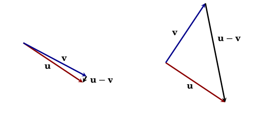
Equation (3.3.2) is the key to the computational attractiveness of orthogonality. Figure 3.3.1 shows how nonorthogonal vectors can allow a multidimensional version of subtractive cancellation, in which $\|\mathbf{x}-\mathbf{y}\|$ is much smaller than $\|\mathbf{x}\|$ and $\|\mathbf{y}\|$ . As the figure illustrates, orthogonal vectors do not allow this phenomenon. By (3.3.2), the magnitude of a vector difference or sum is larger than the magnitudes of the original vectors.

Figure 3.3.1:Nonorthogonal vectors can cause cancellation when subtracted, but orthogonal vectors never do.

3.3.1Orthogonal and ONC matrices¶

Statements about orthogonal vectors are often made more easily in matrix form. Let $\mathbf{Q}$ be an $n\times k$ matrix whose columns $\mathbf{q}_1, \ldots, \mathbf{q}_k$ are orthogonal vectors. The orthogonality conditions (3.3.1) become simply that $\mathbf{Q}^T\mathbf{Q}$ is a diagonal matrix, since

\mathbf{Q}^T \mathbf{Q} = \begin{bmatrix} \mathbf{q}_1^T \\[1mm] \mathbf{q}_2^T \\ \vdots \\ \mathbf{q}_k^T \end{bmatrix} \begin{bmatrix} \mathbf{q}_1 & \mathbf{q}_2 & \cdots & \mathbf{q}_k \end{bmatrix} = \begin{bmatrix} \mathbf{q}_1^T\mathbf{q}_1 & \mathbf{q}_1^T\mathbf{q}_2 & \cdots & \mathbf{q}_1^T\mathbf{q}_k \\[1mm] \mathbf{q}_2^T\mathbf{q}_1 & \mathbf{q}_2^T\mathbf{q}_2 & \cdots & \mathbf{q}_2^T\mathbf{q}_k \\ \vdots & \vdots & & \vdots \\ \mathbf{q}_k^T\mathbf{q}_1 & \mathbf{q}_k^T\mathbf{q}_2 & \cdots & \mathbf{q}_k^T\mathbf{q}_k \end{bmatrix}.

(3.3.3)

If the columns of $\mathbf{Q}$ are orthonormal, then $\mathbf{Q}^T\mathbf{Q}$ is the $k\times k$ identity matrix. This is such an important property that we will break with common practice here and give this type of matrix a name.

Of particular interest is a square ONC matrix.^[1]

Orthogonal matrices have properties beyond Theorem 3.3.1.

3.3.2Orthogonal factorization¶

Now we come to another important way to factor a matrix: the QR factorization. As we will show below, the QR factorization plays a role in linear least squares analogous to the role of LU factorization in linear systems.

In most introductory books on linear algebra, the QR factorization is derived through a process known as Gram–Schmidt orthogonalization. However, while it is an important tool for theoretical work, the Gram–Schmidt process is numerically unstable. We will consider an alternative construction in Computing QR factorizations.

When $m$ is much larger than $n$ , which is often the case, there is a compressed form of the factorization that is more efficient. In the product

\mathbf{A} = \begin{bmatrix} \mathbf{q}_1 & \mathbf{q}_2 & \cdots & \mathbf{q}_m \end{bmatrix} \begin{bmatrix} r_{11} & r_{12} & \cdots & r_{1n} \\ 0 & r_{22} & \cdots & r_{2n} \\ \vdots & & \ddots & \vdots\\ 0 & 0 & \cdots & r_{nn} \\ 0 & 0 & \cdots & 0 \\ \vdots & \vdots & & \vdots \\ 0 & 0 & \cdots & 0 \end{bmatrix},

(3.3.5)

the vectors $\mathbf{q}_{n+1},\ldots,\mathbf{q}_m$ always get multiplied by zero. Nothing about $\mathbf{A}$ is lost if we delete them and reduce the factorization to the equivalent form

\mathbf{A} = \begin{bmatrix} \mathbf{q}_1 & \mathbf{q}_2 & \cdots & \mathbf{q}_n \end{bmatrix} \begin{bmatrix} r_{11} & r_{12} & \cdots & r_{1n} \\ 0 & r_{22} & \cdots & r_{2n} \\ \vdots & & \ddots & \vdots\\ 0 & 0 & \cdots & r_{nn} \end{bmatrix} = \hat{\mathbf{Q}} \hat{\mathbf{R}}.

(3.3.6)

Example 3.3.1 (QR factorization)

NumPy provides access to both the thin and full forms of the QR factorization.

A = 1.0 + floor(9 * random.rand(6,4))
A.shape

(6, 4)

Here is the full form:

from numpy.linalg import qr
Q, R = qr(A, "complete")
print(f"size of Q is {Q.shape}")
print("R:")
print(R)

size of Q is (6, 6)
R:
[[-18.22086716  -5.54309513 -13.11682907 -13.83029676]
 [  0.          -5.50219014   0.12864538  -1.69702412]
 [  0.           0.           5.37887029  -1.33695811]
 [  0.           0.           0.           4.24918153]
 [  0.           0.           0.           0.        ]
 [  0.           0.           0.           0.        ]]

We can test that $\mathbf{Q}$ is an orthogonal matrix:

print(f"norm of (Q^T Q - I) is {norm(Q.T @ Q - eye(6)):.3e}")

norm of (Q^T Q - I) is 7.072e-16

The default for qr, and the one you usually want, is the thin form.

Q_hat, R_hat = qr(A)
print(f"size of Q_hat is {Q_hat.shape}")
print("R_hat:")
print(R_hat)

size of Q_hat is (6, 4)
R_hat:
[[-18.22086716  -5.54309513 -13.11682907 -13.83029676]
 [  0.          -5.50219014   0.12864538  -1.69702412]
 [  0.           0.           5.37887029  -1.33695811]
 [  0.           0.           0.           4.24918153]]

Now $\hat{\mathbf{Q}}$ cannot be an orthogonal matrix, because it is not square, but it is still ONC. Mathematically, $\hat{\mathbf{Q}}^T \hat{\mathbf{Q}}$ is a $4\times 4$ identity matrix.

print(f"norm of (Q_hat^T Q_hat - I) is {norm(Q_hat.T @ Q_hat - eye(4)):.3e}")

norm of (Q_hat^T Q_hat - I) is 4.599e-16

3.3.3Least squares and QR¶

If we substitute the thin factorization (3.3.6) into the normal equations (3.2.3), we can simplify expressions a great deal.

\begin{split} \mathbf{A}^T\mathbf{A} \mathbf{x} &= \mathbf{A}^T \mathbf{b}, \\ \hat{\mathbf{R}}^T \hat{\mathbf{Q}}^T \hat{\mathbf{Q}} \hat{\mathbf{R}} \mathbf{x} &= \hat{\mathbf{R}}^T \hat{\mathbf{Q}}^T \mathbf{b}, \\ \hat{\mathbf{R}}^T \hat{\mathbf{R}} \mathbf{x}& = \hat{\mathbf{R}}^T \hat{\mathbf{Q}}^T \mathbf{b}. \end{split}

(3.3.7)

In order to have the normal equations be well posed, we require that $\mathbf{A}$ is not rank-deficient (as proved in Theorem 3.2.2). This is enough to guarantee that $\hat{\mathbf{R}}$ is nonsingular (see Exercise 3.3.4). Therefore, its transpose is nonsingular as well, and we arrive at

\hat{\mathbf{R}} \mathbf{x}=\hat{\mathbf{Q}}^T \mathbf{b}.

(3.3.8)

This algorithm is implemented in Function 3.3.2. It is essentially the algorithm used internally by Julia when A\b is called. The execution time is dominated by the factorization, the most common method for which is described in Computing QR factorizations.

Algorithm 3.3.2 (lsqrfact)

lsqrfact.py

1
2
3
4
5
6
7
8
9
10
11
def lsqrfact(A, b):
    """
    lsqrfact(A, b)
    
    Solve a linear least squares problem by QR factorization. Returns the
    minimizer of ||b-Ax||.
    """
    Q, R = np.linalg.qr(A)
    c = Q.T @ b
    x = backsub(R, c)
    return x

The solution of least-squares problems via QR factorization is more stable than when the normal equations are formulated and solved directly.

Example 3.3.2 (Stability of least-squares via QR)

We’ll repeat the experiment of Example 3.2.1, which exposed instability in the normal equations.

t = linspace(0, 3, 400)
A = array([ [sin(t)**2, cos((1+1e-7)*t)**2, 1] for t in t ])
x = array([1, 2, 1])
b = A @ x

The error in the solution by Function 3.3.2 is similar to the bound predicted by the condition number.

from numpy.linalg import cond
print(f"observed error: {norm(FNC.lsqrfact(A, b) - x) / norm(x):.3e}")
print(f"conditioning bound: {cond(A) * finfo(float).eps:.3e}")

observed error: 5.186e-09
conditioning bound: 4.053e-09

3.3.4Exercises¶

Footnotes¶

Confusingly, a square matrix whose columns are orthogonal is not necessarily an orthogonal matrix; the columns must be orthonormal, which is a stricter condition.
↩